15 Continuous Random Variables: Probability Density Functions

The continuous analog of a probability mass function (pmf) is a probability density function (pdf).
However, while pmfs and pdfs play analogous roles, they are different in one fundamental way; namely, a pmf outputs probabilities directly, while a pdf does not.
A pdf of a continuous random variable must be integrated to find probabilities of related events.
The probability density function (pdf) (a.k.a. density) of a continuous RV $X$, defined on a probability space with probability measure $\text{P}$, is a function $f_X:\mathbb{R}\mapsto[0,\infty)$ which satisfies \[\begin{align*} \text{P}(a \le X \le b) & =\int_a^b f_X(x) dx, \qquad \text{for all } -\infty \le a \le b \le \infty \end{align*}\]
For a continuous random variable $X$ with pdf $f_X$, the probability that $X$ takes a value in the interval $[a, b]$ is the area under the pdf over the region $[a,b]$.
The axioms of probability imply that a valid pdf must satisfy \[\begin{align*} f_X(x) & \ge 0 \qquad \text{for all } x,\\ \int_{-\infty}^\infty f_X(x) dx & = 1 \end{align*}\]

Example 15.1 Two resistors are randomly selected and connected in series, so that the system resistance $X$ (ohms) is the sum of the two resistances. Assume that the first resistor has a marginal Uniform(135, 165) distribution, and the second has a marginal Uniform(162, 198) distribution (corresponding to nominal 150 and 180 ohm resistors with 10% tolerance). Also assume that the two resistances are independent.

Simulation suggests that the pdf of $X$ is

\[ f_X(x) = \begin{cases} \frac{1}{33}\left(1-\frac{1}{33}|x - 330|\right), & 297 < x < 363\\ 0, & \text{otherwise.} \end{cases} \]

Sketch a plot of the pdf. What does this say about the distribution of the system resistance?
Verify that $f_X$ is a valid pdf.
Find $\text{P}(X > 340)$.
Find $\text{P}(330 < X< 340)$.

15.1 Density is not probability

Example 15.2 Continuing Example 15.1, where the series system resistance $X$ (ohms) has pdf \[ f_X(x) = \begin{cases} \frac{1}{33}\left(1-\frac{1}{33}|x - 330|\right), & 297 < x < 363\\ 0, & \text{otherwise.} \end{cases} \]

Compute $\text{P}(X = 340)$.
Compute the probability that $X$, rounded to one decimal place, is 340.0.
How is the probability in the previous part related to $f_X(340)$?
How many times more likely is $X$, rounded to one decimal place, to be 340.0 than to be 350.0?

The probability that a continuous random variable $X$ equals any particular value is 0. That is, if $X$ is continuous then $\text{P}(X=x)=0$ for all $x$.
For a continuous random variable $X$, $\text{P}(X \le x) = \text{P}(X < x)$, etc.
- Careful: this is NOT true for discrete random variables; for a discrete random variable $\text{P}(X \le x) = \text{P}(X < x) + \text{P}(X = x)$.
For continuous random variables, it doesn’t really make sense to talk about the probability that the random value is equal to a particular value. However, we can consider the probability that a random variable is close to a particular value.
The density $f_X(x)$ at value $x$ is not a probability.
Rather, the density $f_X(x)$ at value $x$ is related to the probability that the RV $X$ takes a value “close to $x$” in the following sense \[ \text{P}\left(x-\frac{\epsilon}{2} \le X \le x+\frac{\epsilon}{2}\right) \approx \epsilon f_X(x), \qquad \text{for small $\epsilon$} \]
The quantity $\epsilon$ is a small number that represents the desired degree of precision. For example, rounding to two decimal places corresponds to $\epsilon=0.01$.
What’s important about a pdf is relative heights. For example, if $f_X(x_2)/ f_X(x_1) = 2$ then $X$ is roughly “twice as likely to be near $x_2$ than to be near $x_1$” in the above sense. \[ \frac{f_X(x_2)}{f_X(x_1)} = \frac{\epsilon f_X(x_2)}{\epsilon f_X(x_1)} \approx \frac{\text{P}\left(x_2-\frac{\epsilon}{2} \le X \le x_2+\frac{\epsilon}{2}\right)}{\text{P}\left(x_1-\frac{\epsilon}{2} \le X \le x_1+\frac{\epsilon}{2}\right)} \]

15.2 Exponential distributions

Example 15.3 Suppose that we model the waiting time, measured continuously in hours, from now until the next earthquake (of any magnitude) occurs in southern CA as a continuous random variable $X$ with pdf \[ f_X(x) = 2 e^{-2x}, \; x \ge0. \] This is the pdf of the “Exponential(2)” distribution.

Sketch the pdf of $X$. What does this tell you about waiting times?
Compute $\text{P}(X = 0.5)$.
Without doing any integration, approximate the probability that $X$ rounded to the nearest minute is 0.5 hours.
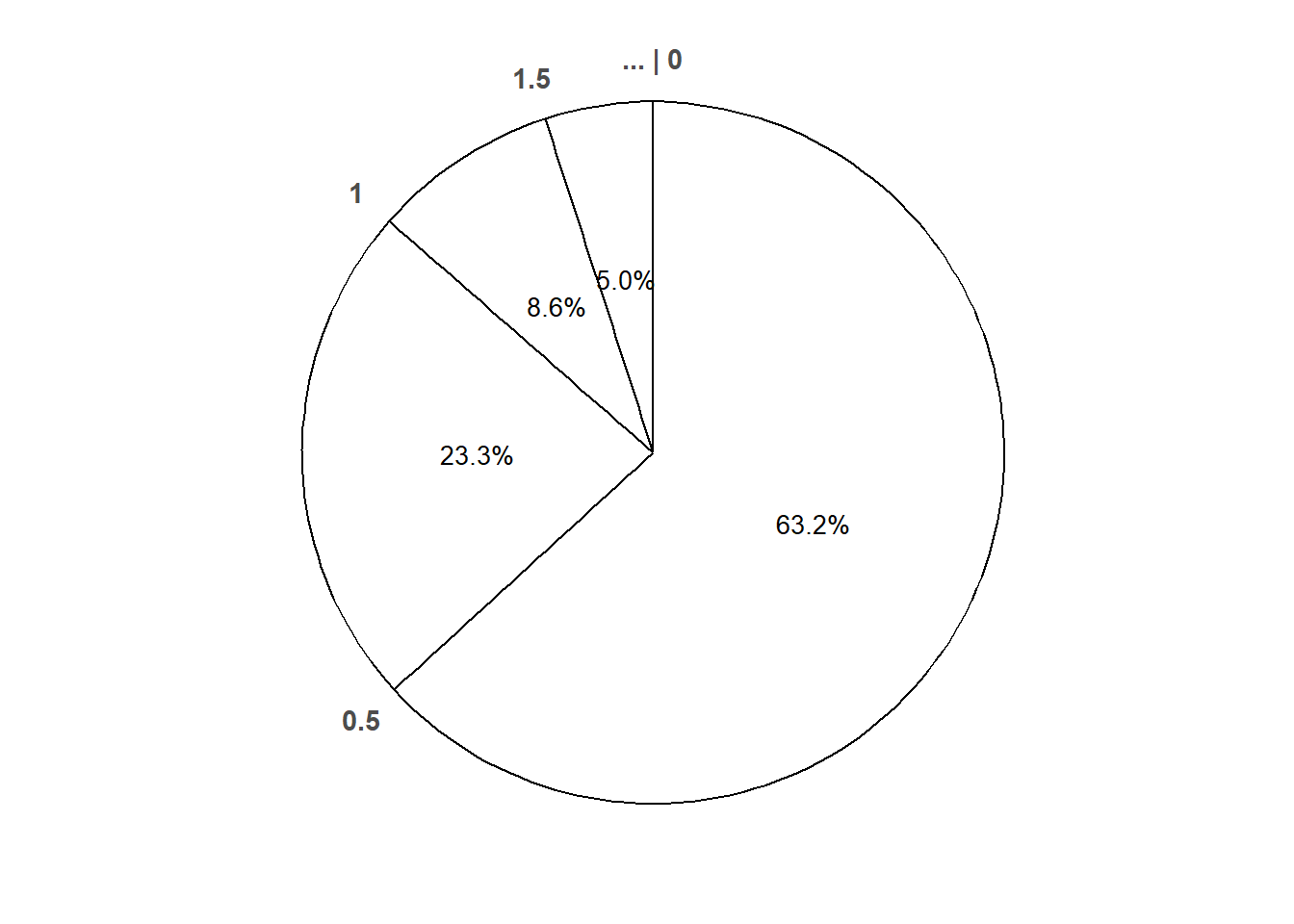
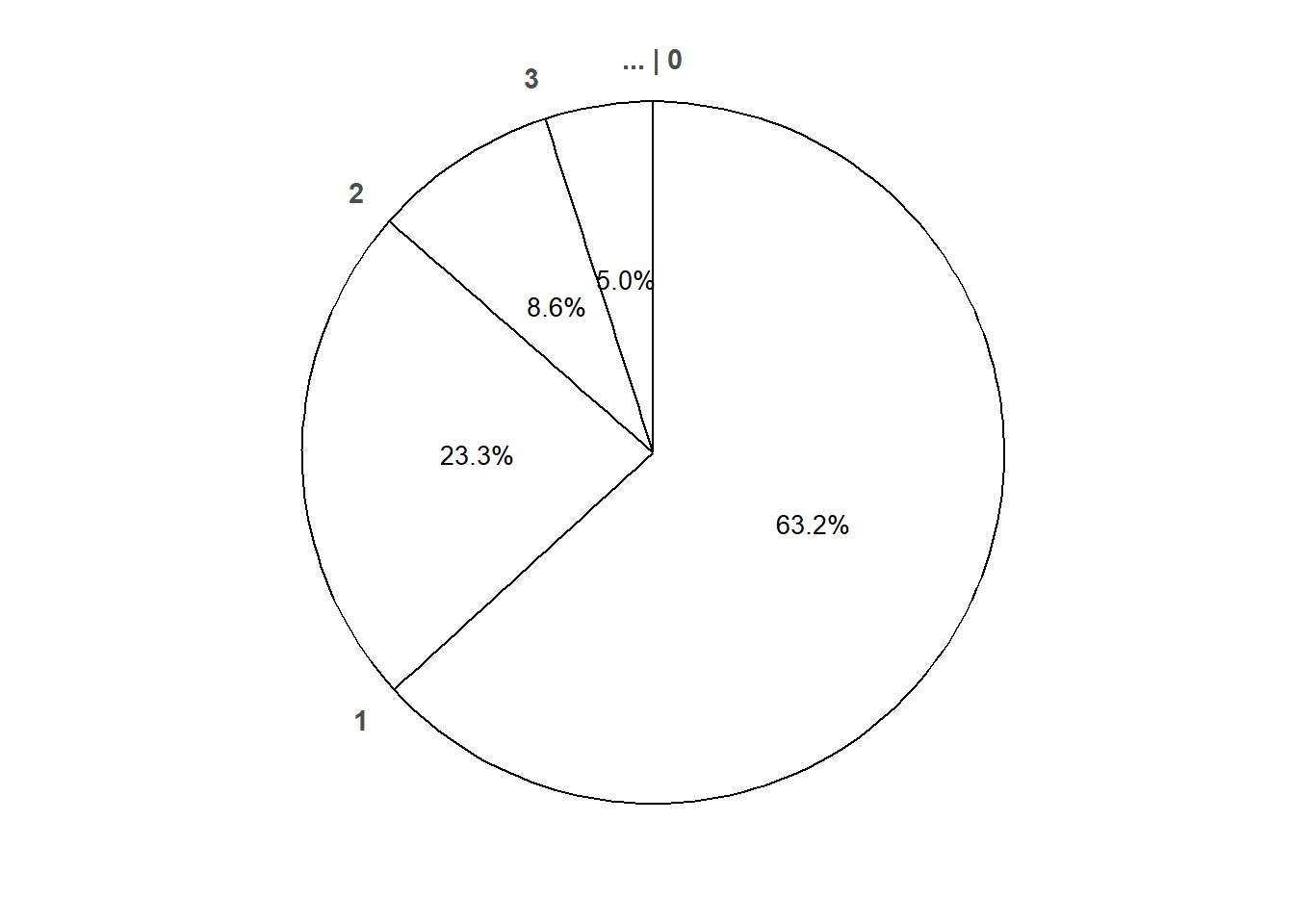
Without doing any integration determine how much more likely is it for $X$ rounded to the nearest minute to be 0.5 than 1.5.
Compute and interpret $\text{P}(X > 0.25)$.
Compute and interpret $\text{P}(X \le 3)$.
Compute and interpret the 25th percentile of $X$.
Compute and interpret the 50th percentile of $X$.
Compute and interpret the 75th percentile of $X$.
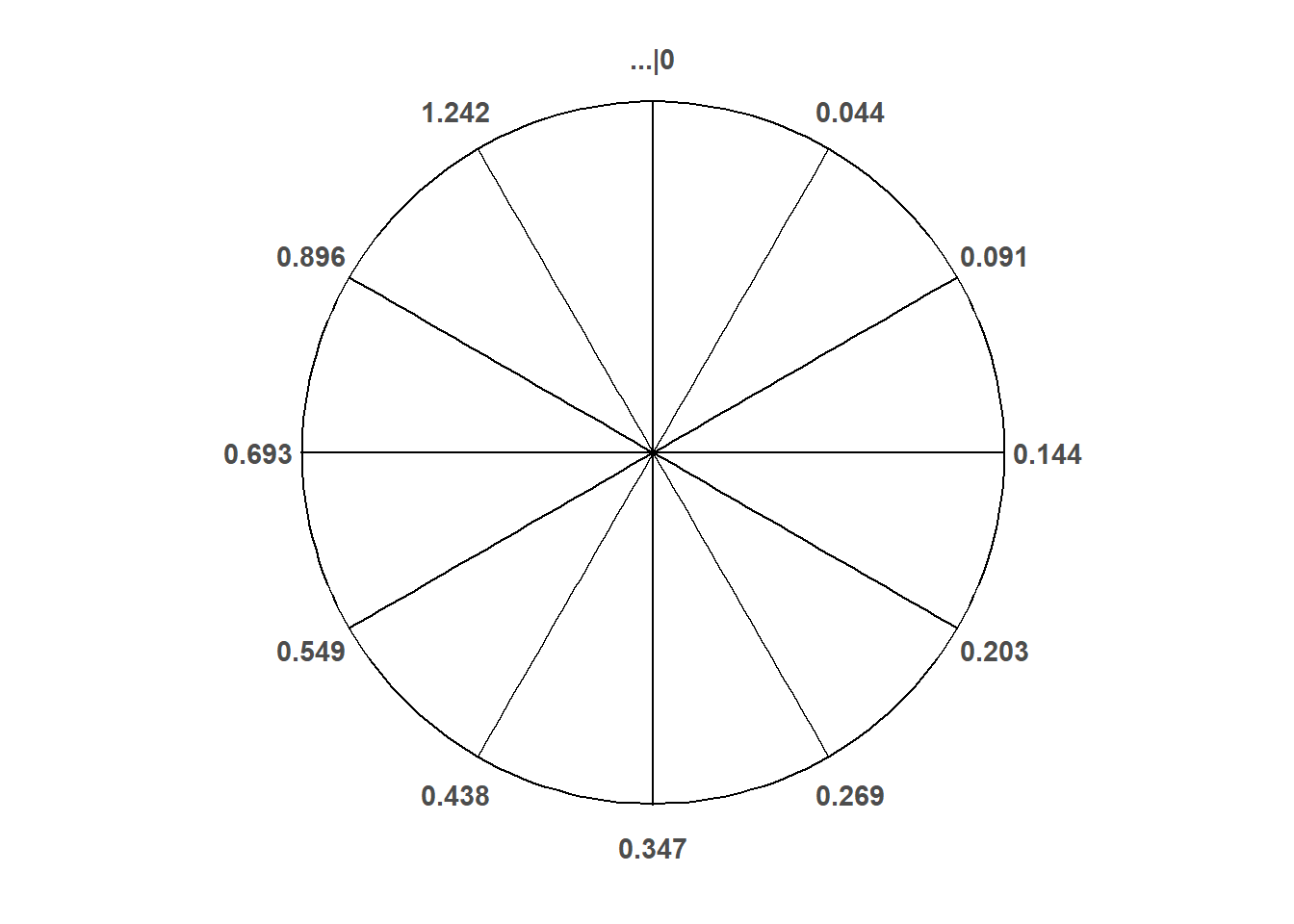
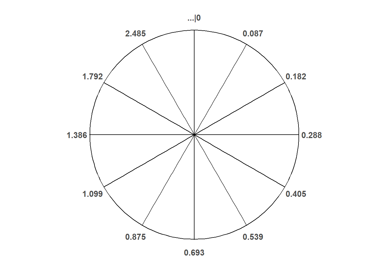
Start to construct a spinner corresponding to this Exponential(2) distribution.
Use simulation to approximate the long run average value of $X$. Interpret this value. At what rate do earthquakes tend to occur?
Use simulation to approximate the standard deviation of $X$. What do you notice?

Exponential distributions are often used to model the waiting times between events in a random process that occurs continuously over time.
A continuous random variable $X$ has an Exponential distribution with rate parameter $\lambda>0$ if its pdf is \[ f_X(x) = \begin{cases}\lambda e^{-\lambda x}, & x \ge 0,\\ 0, & \text{otherwise} \end{cases} \]
If $X$ has an Exponential($\lambda$) distribution then \[\begin{align*} \text{P}(X>x) & = e^{-\lambda x}, \quad x\ge 0\\ \text{Long run average of $X$} & = \frac{1}{\lambda}\\ \text{Standard deviation of $X$} & = \frac{1}{\lambda} \end{align*}\]
Exponential distributions are often used to model the waiting time in a random process until some event occurs.
- $\lambda$ is the average rate at which events occur over time (e.g., 2 per hour)
- $1/\lambda$ is the mean time between events (e.g., 1/2 hour)
The “standard” Exponential distribution is the Exponential(1) distribution, with rate parameter 1 and mean 1.
If $X$ has an Exponential(1) distribution and $\lambda>0$ is a constant then $X/\lambda$ has an Exponential($\lambda$) distribution.

15.3 Uniform distributions

A continuous random variable $X$ has a Uniform distribution with parameters $a$ and $b$, with $a<b$, if its probability density function $f_X$ satisfies \[\begin{align*} f_X(x) & \propto \text{constant}, \quad & & a<x<b\\ & = \frac{1}{b-a}, \quad & & a<x<b. \end{align*}\]
If $X$ has a Uniform($a$, $b$) distribution then \[\begin{align*} \text{Long run average value of $X$} & = \frac{a+b}{2}\\ \text{Variance of $X$} & = \frac{|b-a|^2}{12}\\ \text{SD of $X$} & = \frac{|b-a|}{\sqrt{12}} \end{align*}\]
The “standard” Uniform distribution is the Uniform(0, 1) distribution.
If $U$ has a Uniform(0, 1) distribution then $X = a + (b-a)U$ has a Uniform($a$, $b$) distribution.