34  Gaussian Processes and Brownian Motion

• A stochastic process \(X(t)\) is a Gaussian process if for any time points \(t_1, \ldots, t_n\) the process values \(X(t_1), \ldots, X(t_n)\) have a joint Gaussian (a.k.a. Multivariate Normal) distribution.
• That is, a stochastic process \(X(t)\) is a Gaussian process if for any \(n\) and any time points \(t_1, \ldots, t_n\) any linear combination of the process values \(X(t_1), \ldots, X(t_n)\) has a Normal (Gaussian) distribution.
• In particular, at any time \(t\) the process value \(X(t)\) has a Normal (Gaussian) distribution.
• In particular, at any pair of times \(t\) and \(s\) the pair of process values \((X(t), X(s))\) has a Bivariate Normal (Bivariate Gaussian) distribution.
• The distributional properties of a Gaussian process are completely specified by its:
  • mean function \(\mu_X(t)\), and
  • autocovariance function \(C_{X}(s,t)\) (or autocorrelation function \(R_{X}(s,t)\)).
• If a Gaussian process is WSS then it is strict-sence stationary.
  • Remember, WSS does not imply strict-sense stationary in general.

Example 34.1 The noise in a signal \(X(t)\) is modeled as a Gaussian process with mean 0.9 and autocovariance function \(C_{X}(t,t+\tau)=0.04e^{-0.1|\tau|}\).

1. Is \(X(t)\) a WSS process?
   
   
   
   
   

2. Specify the distribution of \(X(3)\).
   
   
   
   
   

3. Compute \(\text{P}(X(3) > 0.6)\).
   
   
   
   
   

4. Without doing any further calculations, specify the distribution of \(X(t)\), and \(\text{P}(X(t) > 0.6)\), for any \(t\). Explain.
   
   
   
   
   

5. Specify the joint distribution of \(X(3)\) and \(X(8)\).
   
   
   
   
   

6. Determine the probability that the noise at \(t = 3\) seconds is more than 0.5 above the noise at \(s= 8\) seconds.
   
   
   
   
   

7. Compute \(\text{P}(X(3) > 0.6 | X(8) = 0.5)\).
   
   
   
   
   

8. Without doing any calculations, find \(\text{P}(X(3) > 0.3 | X(100) = 0.6)\).
   
   
   
   
   

• A stochastic process \(\{B(t), t\ge 0\}\) is a Brownian motion (process) (a.k.a. Wiener process) with scale parameter \(\alpha\) if:
  • \(B(0)=0\)
  • For all \(t,\tau\ge 0\), \(B(t+\tau)-B(t) \sim N(0,\alpha\sqrt{\tau})\)
    • So Brownian motion has stationary increments
  • For all \(t,\tau\ge 0\), \(B(t+\tau)-B(t)\) is independent of \(\{B(s), 0 \le s \le t\}\)
    • So Brownian motion has independent increments
  • For each outcome, the sample path \(t\mapsto B(t)\) is a continuous¹ function of \(t\).
• A Brownian motion process is a Gaussian process with \[\begin{align*} \text{Mean function:} & & \text{E}(B(t)) & = 0\\ \text{Variance function:} & & \text{Var}(B(t)) & = \alpha^2 t\\ \text{Autocovariance function:} & & \text{Cov}(B(t), B(s)) & = \alpha^2 \min(t, s)\\ \end{align*}\]

The stochastic process represented by Figure 29.1 and Figure 29.2 is a Brownian motion process with scale parameter \(\alpha=1\).

Example 34.2 Brownian motion is often used to model the behavior of charge carriers (electrons and holes) in semiconductors. Suppose that for one particular semiconductor material, the motion of holes is a given direction (say, in microns per second) is Brownian motion with \(\alpha = 100\).

1. What does \(B(3)\) represent?
   
   
   
   
   

2. What does \(B(5)-B(2)\) represent?
   
   
   
   
   

3. Do the symbols \(B(3)\) and \(B(5)-B(2)\) denote the same random variable?
   
   
   
   
   

4. Does \(B(3)\) have the same distribution as \(B(5)\)? If not, state a quantity involving \(B(5)\) that does have the same distribution as \(B(3)\).
   
   
   
   
   

5. Is \(B(3)\) independent of \(B(5)\)? If not, state a quantity involving \(B(5)\) that is independent of \(B(3)\).
   
   
   
   
   

6. Is \(B(3)\) independent of \(B(5) - B(2)\)? If not, state a quantity involving \(B(5)\) that is independent of \(B(3)\).
   
   
   
   
   

7. Compute the probability that a carrier is more than 200 microns from its initial position, in either direction, after 3 seconds.
   
   
   
   
   

8. Compute the probability that at time 5 seconds a carrier is more than 200 microns away, in either direction, from its position at time 2 seconds.
   
   
   
   
   

• Let \(X_1,X_2, \ldots\), be independent with \(\text{P}(X_i=+1)=1/2\) and \(\text{P}(X_i=-1)=1/2\)
• Define \(S_0=0\) and \[ S_n = \sum_{i=1}^n X_i \]
• The discrete-time stochastic process \(\{S_n, n=0,1,2,\ldots\}\) is a symmetric simple random walk (RW).
• Properties of a symmetric simple random walk \[\begin{align*} \text{Mean function:} & & \text{E}(S_n) & = 0\\ \text{Variance function:} & & \text{Var}(S_n) & = n\\ \text{Autocovariance function:} & & \text{Cov}(S_n, S_m) & = \min(n, m)\\ \end{align*}\]
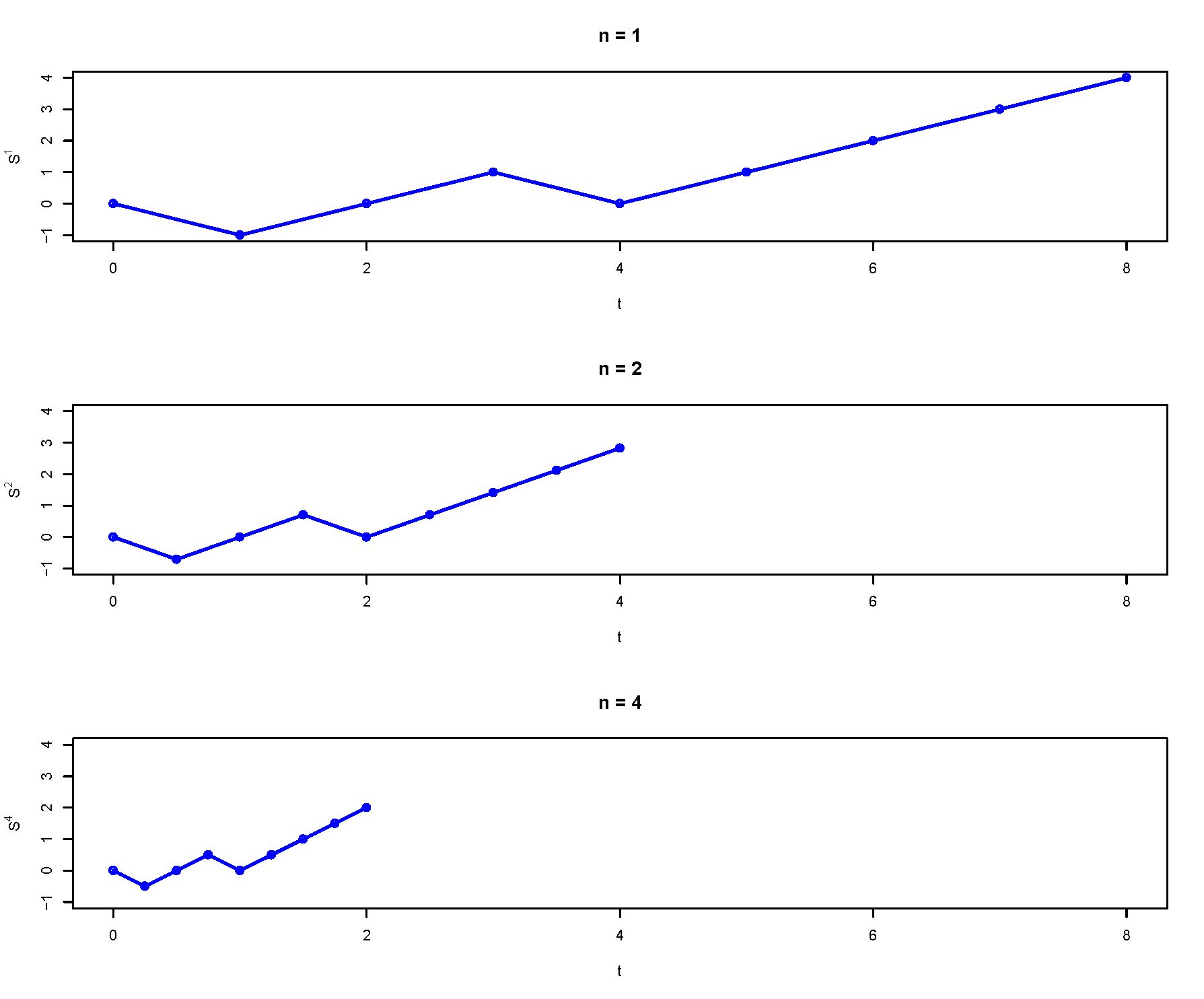
• A Brownian motion process is a continuous — in time and in state — limit of a simple symmetric random walk.
• Continuous path: define for all \(t\ge0\) by “connecting the dots”
• Continuous in time: speed up time between steps by factor of \(n\). (Take a step at times \(1/n,2/n,\ldots\) instead of \(1,2,\ldots)\)
• Continuous in state: scale down size of step by factor² of \(\sqrt{n}\). (Size of step is \(\pm 1/\sqrt{n}\) instead of \(\pm 1\).)
• Take limit as \(n\to\infty\) to get “continuous random walk”, which can be shown to be a Brownian motion process \[ \lim_{n\to\infty}\frac{1}{\sqrt{n}}S_{nt} = B(t) \]

---

1. Fun fact: while every path of Brownian motion is a continuous function of \(t\), it can be shown that every path of Brownian motion is not differentiable for any \(t\).

2. Note: \(\text{E}(|S_n|)=c\sqrt{n}\) so the magnitude of the value of the SSRW after \(n\) steps is on the order of \(\sqrt{n}\). The square root scaling is “just right”; with some other factor the process would either blow up or collapse to 0 in the limit.