10  Conditional Distributions

• The joint distribution of random variables \(X\) and \(Y\) is a probability distribution on \((x, y)\) pairs, and describes how the values of \(X\) and \(Y\) vary together or jointly.
• We can also study conditional distributions of random variables given the values of some random variables. How does the distribution of \(Y\) change for different values of \(X\) (and vice versa)?

Example 10.1 Roll a fair four-sided die twice. Let \(X\) be the sum of the two rolls, and let \(Y\) be the larger of the two rolls (or the common value if a tie). We have previously found the joint and marginal distributions of \(X\) and \(Y\), displayed in the two-way table below.

\((x, y)\)
	1	2	3	4	Total
2	1/16	0	0	0	1/16
3	0	2/16	0	0	2/16
4	0	1/16	2/16	0	3/16
5	0	0	2/16	2/16	4/16
6	0	0	1/16	2/16	3/16
7	0	0	0	2/16	2/16
8	0	0	0	1/16	1/16
Total	1/16	3/16	5/16	7/16

1. Compute \(\text{P}(X=6|Y=4)\).
   
   
   
   
   
2. Construct a table, plot, and spinner to represent the conditional distribution of \(X\) given \(Y=4\).
   
   
   
   
   
3. Construct a table, plot, and spinner to represent the conditional distribution of \(X\) given \(Y=3\).
   
   
   
   
   
4. Construct a table, plot, and spinner to represent the conditional distribution of \(X\) given \(Y=2\).
   
   
   
   
   
5. Construct a table, plot, and spinner to represent the conditional distribution of \(X\) given \(Y=1\).
   
   
   
   
   
6. Compute \(\text{P}(Y=4|X=6)\).
   
   
   
   
   
7. Construct a table, plot, and spinner to represent the distribution of \(Y\) given \(X=6\).
   
   
   
   
   

• The conditional distribution of \(Y\) given \(X=x\) is the distribution of \(Y\) values over only those outcomes for which \(X=x\). It is a distribution on values of \(Y\) only; treat \(x\) as a fixed constant when conditioning on the event \(\{X=x\}\).
• Conditional distributions can be obtained from a joint distribution by slicing and renormalizing. The conditional distribution of \(Y\) given \(X=x\), where \(x\) represents a particular number, can be thought of as:
  • the slice of the joint distribution corresponding to \(X=x\), a distribution on values of \(Y\) alone with \(X=x\) fixed
  • renormalized so that the slice accounts for 100% of the probability over the values of \(Y\)
• The shape of the conditional distribution of \(Y\) given \(X=\) is determined by the shape of the slice of the joint distribution over values of \(Y\) for the fixed \(x\).
• For each fixed \(x\), the conditional distribution of \(Y\) given \(X=x\) is a different distribution on values of the random variable \(Y\). There is not one “conditional distribution of \(Y\) given \(X\)”, but rather a family of conditional distributions of \(Y\) given different values of \(X\).
• Each conditional distribution is a distribution, so we can summarize its characteristics like mean and standard deviation. The conditional mean and standard deviation of \(Y\) given \(X=x\) represent, respectively, the long run average and variability of values of \(Y\) over only \((X, Y)\) pairs with \(X=x\).
• Since each value of \(x\) typically corresponds to a different conditional distribution of \(Y\) given \(X=x\), the conditional mean and standard deviation will typically be functions of \(x\).

Example 10.2 We have already discussed two ways for simulating an \((X, Y)\) pair in the dice rolling example: simulate a pair of rolls and measure \(X\) (sum) and \(Y\) (max), or spin the joint distribution spinner for \((X, Y)\) once.

1. Now describe another way for simulating an \((X, Y)\) pair using the spinners in Example 10.1. (Hint: you’ll need one more spinner in addition to the four from the previous example.)
   
   
   
   
   

2. Describe in detail how you can simulate \((X, Y)\) pairs and use the results to approximate \(\text{P}(X = 6 | Y = 4)\).
   
   
   
   
   

3. Describe in detail how you can simulate \((X, Y)\) pairs and use the results to approximate the conditional distribution of \(X\) given \(Y = 4\).
   
   
   
   
   

4. We have seen that the long run average value of \(X\) is 5. Would you expect the conditional long run average value of \(X\) given \(Y= 4\) to be greater than, less than, or equal to 5? Explain without doing any calculations. What about given \(Y = 2\)?
   
   
   
   
   

5. How could you use simulation to approximate the conditional long run average value of \(X\) given \(Y = 4\)?
   
   
   
   
   

• Rather than directly simulating from a joint distribution, we can simulate an \((X, Y)\) pair in two stages:
  • Simulate a value of \(X\) from its marginal distribution. Call the simulated value \(x\).
  • Given \(x\), simulate a value of \(Y\) from the conditional distribution of \(Y\) given \(X = x\). There will be a different distribution (spinner) for each possible value of \(x\).
• This “marginal then conditional” process is essentially implementing the multiplication rule \[ \text{joint} = \text{conditional}\times\text{marginal} \]
• In many problems a joint distribution is naturally described by specifying the marginal distribution of \(X\) and the family of conditional distributions of \(Y\) given values of \(X\)

Example 10.3 Recall the meeting problem. Let \(R\) be the random variable representing Regina’s arrival time (minutes after noon), and \(Y\) for Cady. Assume that they each arrive uniformly at random at a time between noon and 1:00, independently of each other. Let \(T = \min(R, Y)\) be the time at which the first person arrives, and \(W=|R-Y|\) be the amount of time the first person waits for the second to arrive. Recall that we used simulation to see the joint distribution of \(T\) and \(W\) was uniform over the triangular region bounded by \(0<T<60\), \(0<W<60\), and \(T+W<60\).

1. Sketch a plot of the conditional distribution of \(W\) given \(T=15\).
   
   
   
   
   

2. Sketch a plot of the conditional distribution of \(W\) given \(T=45\).
   
   
   
   
   

3. Sketch a plot of the conditional distribution of \(T\) given \(W=15\).
   
   
   
   
   

4. What is the long run average value of \(W\) given \(T=15\)? What is the long run average value of \(W\) given \(T=45\)? How does the long run average value of \(W\) given \(T=t\) depend on the value of \(t\)?
   
   
   
   
   

5. How does the standard deviation of \(W\) given \(T=t\) change as \(t\) increases from 0 to 60?
   
   
   
   
   

Example 10.4 Consider the case of the meeting problem which assumes that the \((R, Y)\) pairs of arrival times follow a Bivariate Normal distribution with means (30, 30), standard deviations (10, 10) and correlation 0.7.

Provide answers to the following questions without doing any calculations. It helps to think of the “long run” here as Regina and Cady meeting for lunch each day over many days.

Figure 10.1: Representation of the joint distribution in Example 10.4. The orange vertical strip represents conditioning on \(R=40\); the pink vertical strip to \(R=15\).

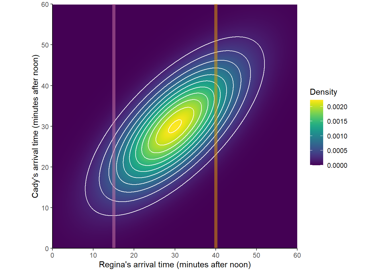
1. Interpret \(\text{P}(Y < 30 | R = 40)\) in context. Is \(\text{P}(Y < 30 | R = 40)\) greater than, less than, or equal to \(\text{P}(Y < 30)\)?
   
   
   
   
   

2. Interpret \(\text{P}(Y < 30 | R = 15)\) in context. Is \(\text{P}(Y < 30 | R = 15)\) greater than, less than, or equal to \(\text{P}(Y < 30)\)?
   
   
   
   
   

3. Interpret \(\text{P}(Y < R | R = 40)\) in context. Is \(\text{P}(Y < R | R = 40)\) greater than, less than, or equal to \(\text{P}(Y < R)\)?
   
   
   
   
   

4. Interpret the conditional long run average value of \(Y\) given \(R= 40\) in context. Is it greater than, less than, or equal to 30 (the long run average value of \(Y\))?
   
   
   
   
   

5. Interpret the conditional long run average value of \(Y\) given \(R= 15\) in context. Is it greater than, less than, or equal to 30 (the long run average value of \(Y\))?
   
   
   
   
   

6. Interpret the conditional standard deviation of \(Y\) given \(R= 40\) in context. Is it greater than, less than, or equal to 10 (the standard deviation of \(Y\))?
   
   
   
   
   

7. Interpret the conditional standard deviation of \(Y\) given \(R= 15\) in context. Is it greater than, less than, or equal to 10 (the standard deviation of \(Y\))?
   
   
   
   
   

8. Sketch a plot of the conditional distribution of \(Y\) given \(R=40\).
   
   
   
   
   

9. Sketch a plot of the conditional distribution of \(Y\) given \(R=15\).
   
   
   
   
   

Example 10.5 Donny Don’t writes the following Symbulate code to approximate the conditional distribution of \(Y\) given \(R=40\), the conditional distribution of Cady’s arrival time given Regina arrives at 12:40. What do you think will happen when Donny runs his code?

R, Y = RV(BivariateNormal(mean1 = 30, sd1 = 10, mean2 = 30, sd2 = 10, corr = 0.7))

(Y | (R == 40) ).sim(10000)

• Be careful when conditioning with continuous random variables. Remember that the probability that a continuous random variable is equal to a particular value is 0; that is, for continuous \(X\), \(\text{P}(X=x)=0\).
• Mathematically, when we condition on \(\{X=x\}\) we are really conditioning on \(\{|X-x|<\epsilon\}\) — the event that the random variable \(X\) is within \(\epsilon\) of the value \(x\) — and seeing what happens in the idealized limit when \(\epsilon\to0\).
• Practically, \(\epsilon\) represents our “close enough” degree of precision, e.g., \(\epsilon=0.01\) if “within 0.01” is close enough.
• When conditioning on a continuous random variable \(X\) in a simulation, never condition on \(\{X=x\}\); rather, condition on \(\{|X-x|<\epsilon\}\) where \(\epsilon\) represents the suitable degree of precision.

Example 10.6 In the meeting problem, assume that \(R\) follows a Normal(30, 10) distribution. For any value \(r\), assume that the conditional distribution of \(Y\) given \(R=r\) is a Normal distribution with mean \(30 + 0.7(r - 30)\) and standard deviation 7.14 minutes.

1. How can we simulate a value of \(R\) using only the standard Normal spinner?
   
   
   
   
   

2. Suppose the simulated value of \(R\) is 40. What is the distribution that we want to simulate the corresponding \(Y\) value from? How can we simulate a value of \(Y\) from this distribution using only the standard Normal spinner?
   
   
   
   
   

3. Now suppose the simulated value of \(R\) is 15. What is the distribution that we want to simulate the corresponding \(Y\) value from? How can we simulate a value of \(Y\) from this distribution using only the standard Normal spinner?
   
   
   
   
   

4. Suggest a general method for simulating an \((R, Y)\) pair.
   
   
   
   
   

5. Simulate many \((R, Y)\) pairs and summarize the results, including the correlation. How does the simulated joint distribution compare to the Bivariate Normal distribution from Example 10.4?
   
   
   
   
   

6. What is the approximate marginal distribution of \(Y\)?
   
   
   
   
   

10.1 Joint, conditional, and marginal distributions

Be sure to distinguish between joint, conditional, and marginal distributions.

• The joint distribution of \(X\) and \(Y\) is a distribution on \((X, Y)\) pairs. A mathematical expression of a joint distribution is a function of both values of \(X\) and values of \(Y\).
• The conditional distribution of \(Y\) given \(X=x\) is a distribution on \(Y\) values (among \((X, Y)\) pairs with a fixed value of \(X=x\)). A mathematical expression of a conditional distribution will involve both \(x\) and \(y\), but \(x\) is treated like a fixed constant and \(y\) is treated as the variable. Note: the possible values of \(Y\) might depend on the value of \(x\).
• The marginal distribution of \(Y\) is a distribution on \(Y\) values only, regardless of the value of \(X\). A mathematical expression of a marginal distribution will have only values of the single variable in it; for example, an expression for the marginal distribution of \(Y\) will only have \(y\) in it (no \(x\), not even in the possible values).