STAT 350 Handouts - 7 Averages and Standard Deviation

7.1 Averages

The marginal distribution of a random variable describes its long run pattern of variability.
One summary characteristic of a distribution is the long run average value of the random variable.
We can approximate the long run average value by simulating many values of the random variable and computing the average (a.k.a., mean) in the usual way.

Example 7.1 Let $X$ be the sum of two rolls of a fair four-sided die, and let $Y$ be the larger of the two rolls (or the common value if a tie). Recall your tactile simulation from Example 5.3.

Based only on the results of your simulation, approximate the long run average value of each of the following: $X$, $Y$, $Y^2$, $XY$. (Don’t worry if the approximations are any good yet.)
Donny Don’t says: “Why bother creating columns for $X^2$ and $XY$? If I want to find the average value of $Y^2$ I can just square the average value of $Y$. For the average value of $XY$ I can just multiply the average value of $X$ and the average value of $Y$.” Do you agree? (Check to see if this works for your simulation results.) If not, explain why not.

In general the order of transforming and averaging is not interchangeable.
Whether in the short run or the long run, in general \[\begin{align*} \text{Average of $g(X)$} & \neq g(\text{Average of $X$})\\ \text{Average of $g(X, Y)$} & \neq g(\text{Average of $X$}, \text{Average of $Y$}) \end{align*}\]
However, the order is interchangeable for linear transformations.
Linearity of averages.: If $X$ and $Y$ are random variables and $a$ and $b$ are non-random constants, whether in the short run or the long run, \[\begin{align*} \text{Average of } (a+bX) & = a+b(\text{Average of } X)\\ \text{Average of } (X+Y) & = \text{Average of } X +\text{Average of } Y \end{align*}\]
The average of the sum of $X$ and $Y$ is the sum of the average of $X$ and the average of $Y$ regardless of the relationship between $X$ and $Y$.

7.2 Standard deviation

The long run average value is just one feature of a distribution.
Random variables vary, and the distribution describes the entire pattern of variability.
We can summarize this degree of variability by listing some percentiles (10th, 25th, 50th, 75th, 90th, etc); the more percentiles we provide the clearer the picture, but the less of a summary.
Standard deviation measures overall degree of variability in a single number as, roughly, the average distance from the mean.
Technically, the variance is the long run average squared distance from the mean, and the standard deviation is the square root of the variance.

\[\begin{align*} \text{Variance of } X & = \text{Average of } ((X - \text{Average of } X)^2)\\ \text{Standard deviation of } X & = \sqrt{\text{Variance of } X} \end{align*}\]

Example 7.2 The plots in Figure 7.1 summarize hypothetical distributions of quiz scores in six classes. All plots are on the same scale. Each quiz score is a whole number between 0 and 10 inclusive.

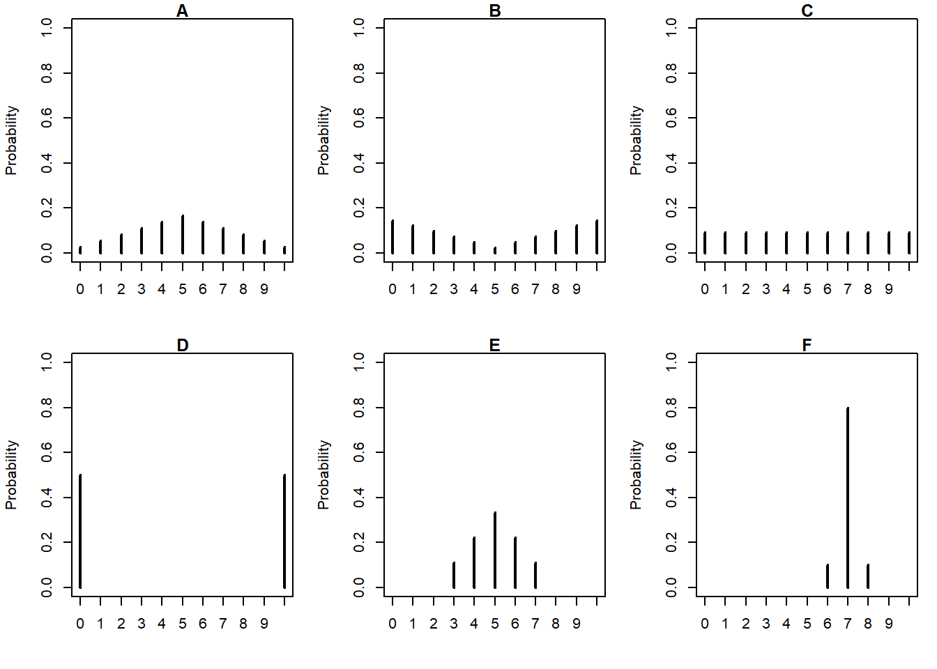
Figure 7.1: A few discrete distributions.

Donny Dont says that C represents the smallest SD, since there is no variability in the heights of the bars. Do you agree that C represents “no variability”? Explain.
What is the smallest possible value the SD of quiz scores could be? What would need to be true about the distribution for this to happen? (This scenario might not be represented by one the plots.)
Without doing any calculations, arrange the classes in order based on their SDs from smallest to largest.
In one of the classes, the SD of quiz scores is 5. Which one? Why?
Is the SD in F greater than, less than, or equal to 1? Why?
Provide a ballpark estimate of the SD in each case.
Consider class E in which the mean is 5 and the SD is 1.15. Suppose the quiz scores were curved by adding 5 to each quiz score (so that the mean becomes 10, and that scores over 10 are allowed). How would the SD change?
Consider class E in which the mean is 5 and the SD is 1.15. Suppose the quiz scores were curved by multiplying each quiz score by 2 (so that the mean becomes 10, and that scores over 10 are allowed). How would the SD change?

If $X$ is a random variable and $a$ and $b$ are non-random constants, whether in the short run or the long run,

\[ \text{SD of } (a+bX) = |b|(\text{SD of } X) \]

Example 7.3 We’ll compare long run average and standard deviation for the Uniform(0, 60) distribution and the Normal(30, 10) distribution. A Normal(30, 10) distribution mean (long run average) 30 and standard deviation 10.

Make an educated guess for the long run average value of a Uniform(0, 60) distribution. Explain.
Will the standard deviation for a Uniform(0, 60) distribution be greater than, less than, or equal to 10, the standard deviation for a Normal(30, 10) distribution? Explain without doing any calculations.
Make an educated guess for the standard deviation of a Uniform(0, 60) distribution.

7.3 Standardization

Standard deviation provides a “ruler” by which we can judge a particular realized value of a random variable relative to the distribution of values.
Standardization measures values in terms of “standard deviations away from the mean”
This idea is particularly useful when comparing random variables with different measurement units but whose distributions have similar shapes. \[ \text{Standardized value} = \frac{\text{Value - Mean}}{\text{Standard deviation}} \]

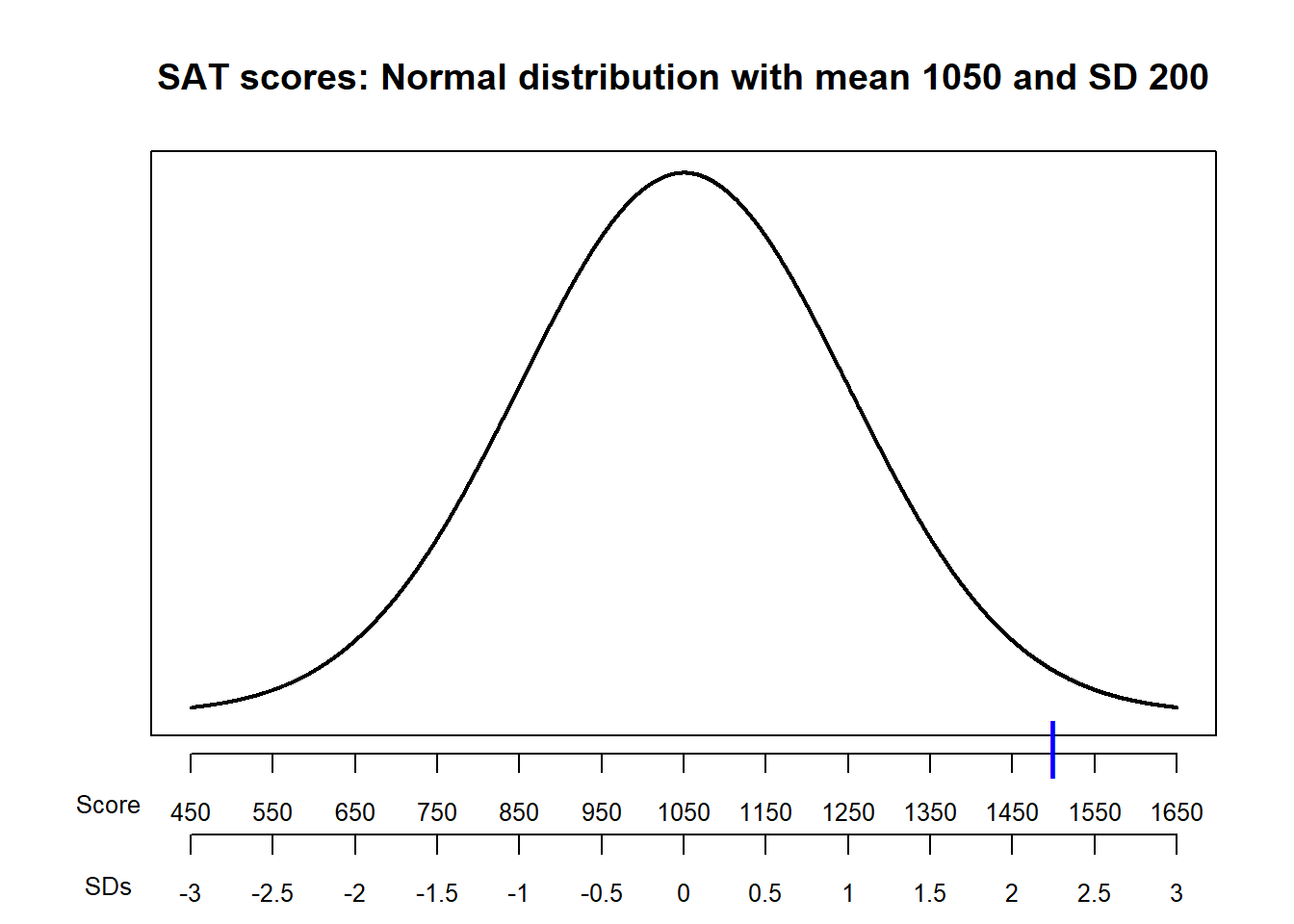
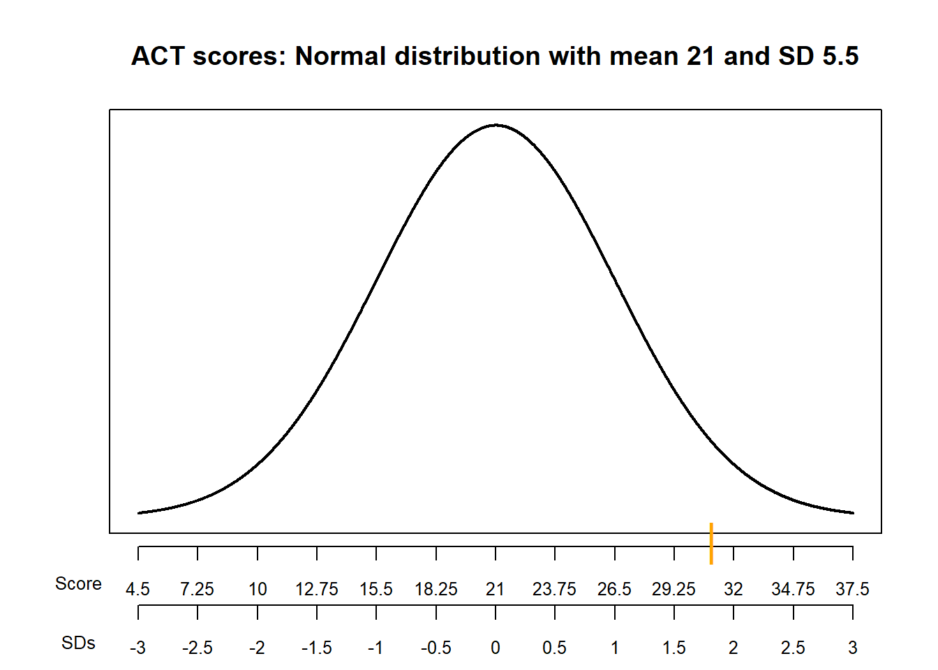
Example 7.4 SAT scores have, approximately, a Normal distribution with a mean of 1050 and a standard deviation of 200. ACT scores have, approximately, a Normal distribution with a mean of 21 and a standard deviation of 5.5. Darius’s score on the SAT is 1500. Alfred’s score on the ACT is 31. Who scored relatively better on their test?

Compute the deviation from the mean for Darius’s SAT score. How does this compare to the average deviation from the mean for SAT scores?
Compute the deviation from the mean for Alfred’s ACT score. How does this compare to the average deviation from the mean for ACT scores?
Who scored relatively better on their test?

(a) The blue mark indicates Darius’s SAT score.

7.4 Normal distributions

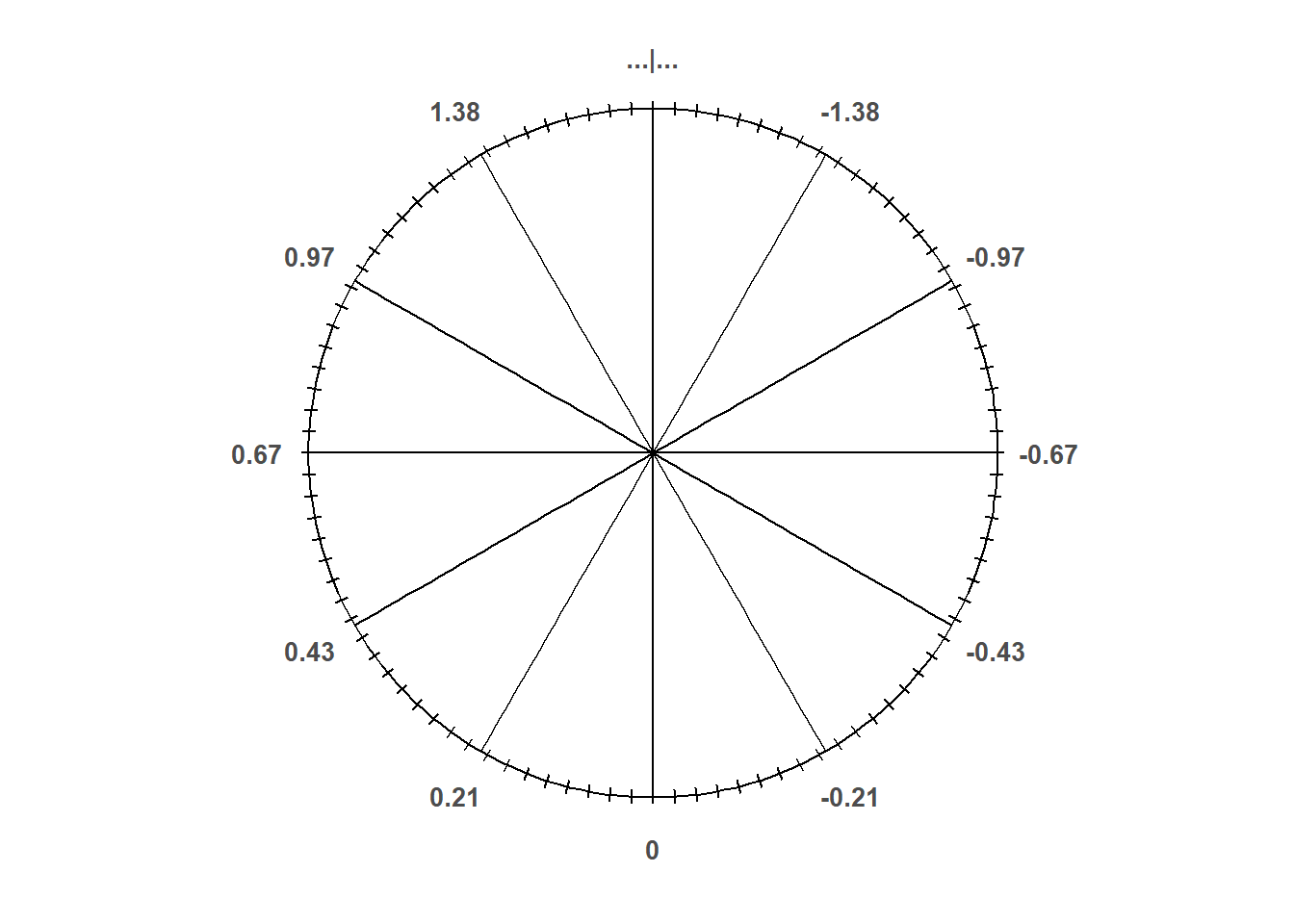
Any Normal distribution follows the “empirical rule” which determines the percentiles that give a Normal distribution its particular bell shape.
For a Normal distribution:
- 50% of values are within 0.67 standard deviations of the mean
- 68% of values are within 1 standard deviation of the mean
- 95% of values are within 2 standard deviations of the mean
- 99.7% of values are within 3 standard deviations of the mean
The table below lists some percentiles of a Normal distribution.

Empirical rule for Normal distributions
Percentile	SDs away from the mean
0.1%	3.09 SDs below the mean
0.5%	2.58 SDs below the mean
1%	2.33 SDs below the mean
2.5%	1.96 SDs below the mean
10%	1.28 SDs below the mean
15.9%	1 SDs below the mean
25%	0.67 SDs below the mean
30.9%	0.5 SDs below the mean
50%	0 SDs above the mean
69.1%	0.5 SDs above the mean
75%	0.67 SDs above the mean
84.1%	1 SDs above the mean
90%	1.28 SDs above the mean
97.5%	1.96 SDs above the mean
99%	2.33 SDs above the mean
99.5%	2.58 SDs above the mean
99.9%	3.09 SDs above the mean

A Normal distribution is determined by its mean and SD; a Normal($\mu$, $\sigma$) distribution has mean $\mu$ and standard deviation $\sigma>0$.
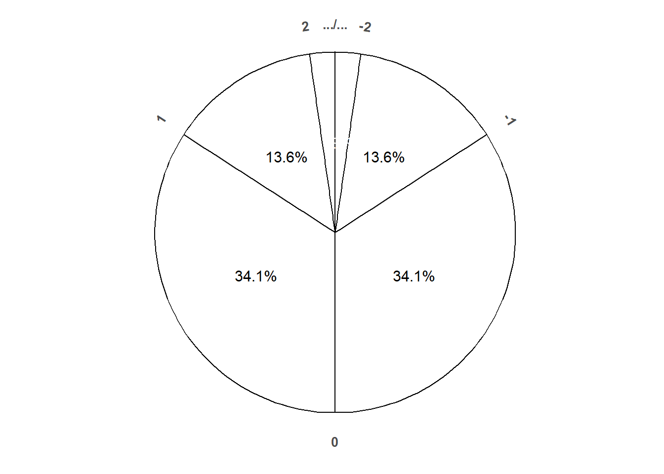
The “standard” Normal distribution is a Normal(0, 1) distribution, with a mean 0 and a standard deviation of 1.
Figure 7.3 corresponds a standard Normal distribution; notice how the spinner reflects the empirical rule.
If $Z$ has a Normal(0, 1) distribution, then $X=\mu + \sigma Z$ has a Normal($\mu$, $\sigma$) distribution (with mean $\mu$ and SD $\sigma$.)

Example 7.5 In a large class, scores on midterm 1 follow (approximately) a Normal$(\mu_1, \sigma)$ distribution and scores on midterm 2 follow (approximately) a Normal$(\mu_2, \sigma)$ distribution. Note that the SD $\sigma$ is the same on both exams. The 25th percentile of midterm 1 scores is equal to the 90th percentile of midterm 2 scores. Compute and interpret

\[ \frac{\mu_1-\mu_2}{\sigma} \]

(This is one statistical measure of effect size.) Note: you do not need to compute $\mu_1$, $\mu_2$, $\sigma$ individually.