27  Normal Distributions

• Normal distributions are probably the most important distributions in probability and statistics.
• Any Normal distribution follows the “empirical rule” which determines the percentiles that give a Normal distribution its particular bell shape. For example,
  • 38% of values are within 0.5 standard deviations of the mean
  • 50% of values are within 0.67 standard deviations of the mean
  • 68% of values are within 1 standard deviation of the mean
  • 87% of values are within 0.5 standard deviations of the mean
  • 95% of values are within 2 standard deviations of the mean
  • 99% of values are within 2.6 standard deviations of the mean
  • 99.7% of values are within 3 standard deviations of the mean

Empirical rule for Normal distributions

Percentile	SDs away from the mean
0.1%	3.09 SDs below the mean
0.5%	2.58 SDs below the mean
1%	2.33 SDs below the mean
2.5%	1.96 SDs below the mean
10%	1.28 SDs below the mean
15.9%	1 SDs below the mean
25%	0.67 SDs below the mean
30.9%	0.5 SDs below the mean
50%	0 SDs above the mean
69.1%	0.5 SDs above the mean
75%	0.67 SDs above the mean
84.1%	1 SDs above the mean
90%	1.28 SDs above the mean
97.5%	1.96 SDs above the mean
99%	2.33 SDs above the mean
99.5%	2.58 SDs above the mean
99.9%	3.09 SDs above the mean

• A continuous random variable \(Z\) has a Standard Normal distribution if its pdf is \[\begin{align*} \phi(z) & = \frac{1}{\sqrt{2\pi}}\,e^{-z^2/2}, \quad -\infty<z<\infty,\\ & \propto e^{-z^2/2}, \quad -\infty<z<\infty. \end{align*}\]
• If \(Z\) has a Standard Normal distribution then \[\begin{align*} \text{E}(Z) & = 0\\ \text{SD}(Z) & = 1 \end{align*}\]
• The Standard Normal pdf is symmetric about its mean of 0, and the peak of the density occurs at 0.
• The standard deviation is 1, and 1 also indicates the distance from the mean to where the concavity of the density changes. That is, there are inflection points at \(\pm1\).
• A continuous random variable \(X\) has a Normal (a.k.a., Gaussian) distribution with mean \(\mu\in (-\infty,\infty)\) and standard deviation \(\sigma>0\) if its pdf is \[\begin{align*} f_X(x) & = \frac{1}{\sigma\sqrt{2\pi}}\,\exp\left(-\frac{1}{2}\left(\frac{x-\mu}{\sigma}\right)^2\right), \quad -\infty<x<\infty,\\ & \propto \exp\left(-\frac{1}{2}\left(\frac{x-\mu}{\sigma}\right)^2\right), \quad -\infty<x<\infty. \end{align*}\]
• If \(X\) has a Normal(\(\mu\), \(\sigma\)) distribution then \[\begin{align*} \text{E}(X) & = \mu\\ \text{SD}(X) & = \sigma \end{align*}\]
• A Normal density is a particular “bell-shaped” curve which is symmetric about its mean \(\mu\). The mean \(\mu\) is a location parameter: \(\mu\) indicates where the center and peak of the distribution is.
• The standard deviation \(\sigma\) is a scale parameter: \(\sigma\) indicates the distance from the mean to where the concavity of the density changes. That is, there are inflection points at \(\mu\pm \sigma\).

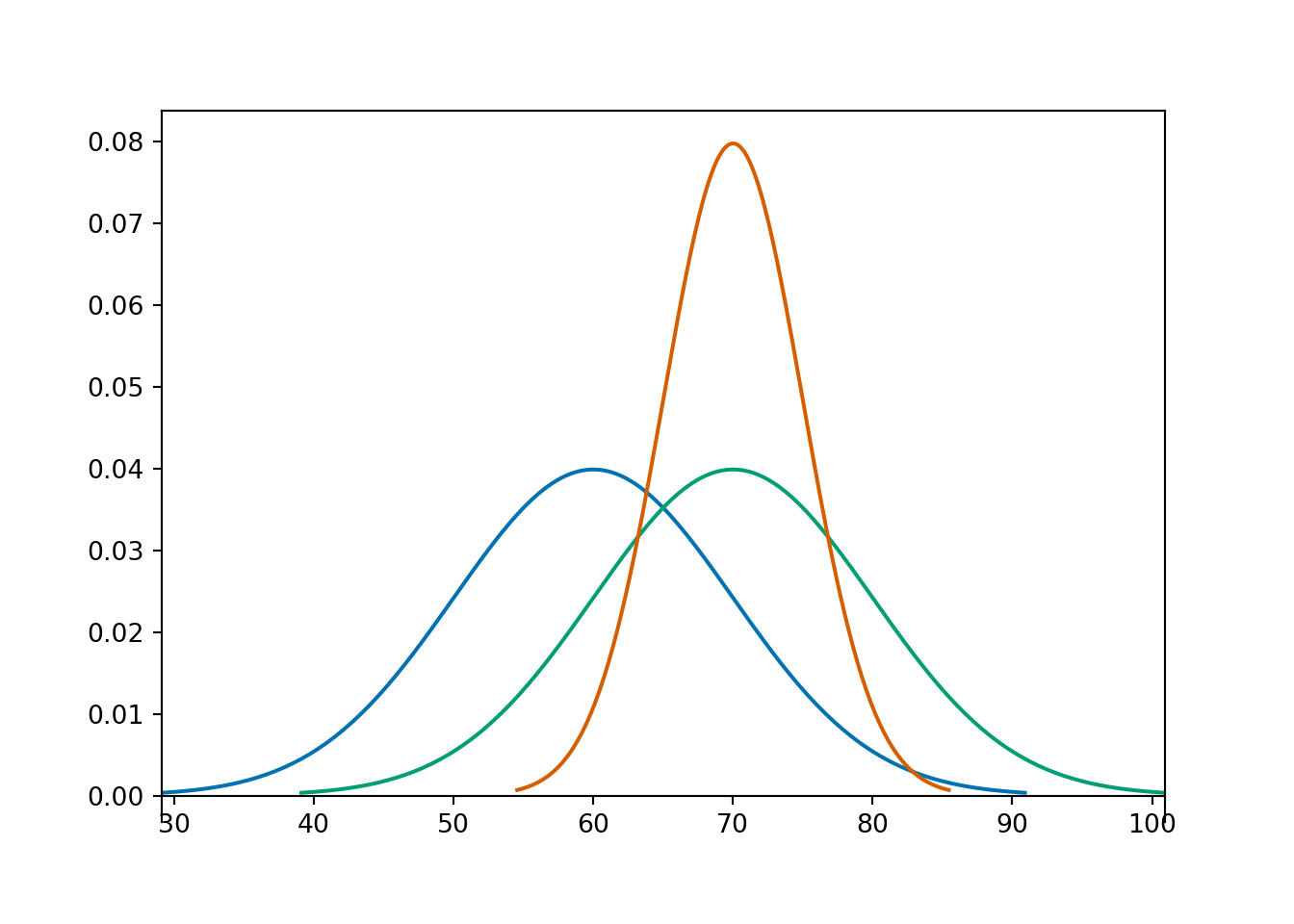
Example 27.1 The pdfs in the plot below represent the distribution of hypothetical test scores in three classes. The test scores in each class follow a Normal distribution. Identify the mean and standard deviation for each class.

Example 27.2 Daily high temperatures (degrees Fahrenheit) in San Luis Obispo in August follow (approximately) a Normal distribution with a mean of 76.9 degrees F. The temperature exceeds 100 degrees Fahrenheit on about 1.5% of August days.

1. What is the standard deviation?
   
   
   
   
   

2. Suppose the mean increases by 2 degrees Fahrenheit. On what percentage of August days will the daily high temperature exceed 100 degrees Fahrenheit? (Assume the standard deviation does not change.)
   
   
   
   
   

3. A mean of 78.9 is 1.02 times greater than a mean of 76.9. By what (multiplicative) factor has the percentage of 100-degree days increased? What do you notice?
   
   
   
   
   

4. If the mean is 76.9, what is the 25th percentile of daily temperatues?
   
   
   
   
   

27.1 Bivariate Normal distributions

• Jointly continuous random variables \(X\) and \(Y\) have a Bivariate Normal distribution with parameters \(\mu_X\), \(\mu_Y\), \(\sigma_X>0\), \(\sigma_Y>0\), and \(-1<\rho<1\) if the joint pdf is, for \(-\infty <x<\infty, -\infty<y<\infty\), \[\begin{align*} f_{X, Y}(x,y) & = \frac{1}{2\pi\sigma_X\sigma_Y\sqrt{1-\rho^2}}\exp\left(-\frac{1}{2(1-\rho^2)}\left[\left(\frac{x-\mu_X}{\sigma_X}\right)^2+\left(\frac{y-\mu_Y}{\sigma_Y}\right)^2-2\rho\left(\frac{x-\mu_X}{\sigma_X}\right)\left(\frac{y-\mu_Y}{\sigma_Y}\right)\right]\right) \end{align*}\]
• It can be shown that if the pair \((X, Y)\) has a BivariateNormal(\(\mu_X\), \(\mu_Y\), \(\sigma_X\), \(\sigma_Y\), \(\rho\)) distribution \[\begin{align*} \text{E}(X) & =\mu_X\\ \text{E}(Y) & =\mu_Y\\ \text{SD}(X) & = \sigma_X\\ \text{SD}(Y) & = \sigma_Y\\ \text{Corr}(X, Y) & = \rho \end{align*}\]
• A Bivariate Normal Density has elliptical contours. For each height \(c>0\) the set \(\{(x,y): f_{X, Y}(x,y)=c\}\) is an ellipse. The density decreases as \((x, y)\) moves away from \((\mu_X, \mu_Y)\), most steeply along the minor axis of the ellipse, and least steeply along the major of the ellipse.
• A scatterplot of \((x,y)\) pairs generated from a Bivariate Normal distribution will have a rough linear association and the cloud of points will resemble an ellipse.
• If \(X\) and \(Y\) have a Bivariate Normal distribution, then the marginal distributions are also Normal: \(X\) has a Normal\(\left(\mu_X,\sigma_X\right)\) distribution and \(Y\) has a Normal\(\left(\mu_Y,\sigma_Y\right)\).
• If \(X\) and \(Y\) have a Bivariate Normal distribution and \(\text{Corr}(X, Y)=0\) then \(X\) and \(Y\) are independent. (Remember, in general it is possible to have situations where the correlation is 0 but the random variables are not independent.)
• It can also be shown that if \(X\) and \(Y\) have a Bivariate Normal distribution then any conditional distribution is Normal. The conditional distribution of \(Y\) given \(X=x\) is \[ N\left(\mu_Y + \frac{\rho\sigma_Y}{\sigma_X}\left(x-\mu_X\right),\;\sigma_Y\sqrt{1-\rho^2}\right) \]
• The conditional expected value of \(Y\) given \(X=x\) is a linear function of \(x\), called the regression line of \(Y\) on \(X\): \[ \text{E}(Y | X=x) = \mu_Y + \rho\sigma_Y\left(\frac{x-\mu_X}{\sigma_X}\right) \]
  • The regression line passes through the point of means \((\mu_X, \mu_Y)\) and has slope \[ \frac{\rho \sigma_Y}{\sigma_X} \]
  • The regression line estimates that if the given \(x\) value is \(z\) SDs above of the mean of \(X\), then the corresponding \(Y\) values will be, on average, \(\rho z\) SDs away from the mean of \(Y\) \[ \frac{\text{E}(Y|X=x) - \mu_Y}{\sigma_Y} = \rho\left(\frac{x-\mu_X}{\sigma_X}\right) \]
  • Since \(|\rho|\le 1\), for a given \(x\) value the corresponding \(Y\) values will be, on average, relatively closer to the mean of \(Y\) than the given \(x\) value is to the mean of \(X\). This is known as regression to the mean.
• For Bivariate Normal distributions, the conditional variance of \(Y\) given \(X=x\) does not depend on \(x\): \[ \text{SD}(Y |X = x) = \sigma_Y\sqrt{1-\rho^2} \]
• \(X\) and \(Y\) have a Bivariate Normal distribution if and only if every linear combination of \(X\) and \(Y\) has a Normal distribution. That is, \(X\) and \(Y\) have a Bivariate Normal distribution if and only if \(aX+bY+c\) has a Normal distribution for all \(a\), \(b\), \(c\).

Example 27.3 Suppose that SAT Math (\(M\)) and Reading (\(R\)) scores of CalPoly students have a Bivariate Normal distribution. Math scores have mean 640 and SD 80, Reading scores have mean 610 and SD 70, and the correlation between scores is 0.7.

1. Find the probability that a student has a Math score above 700.
   
   
   
   
   

2. Find the probability that a student has a total score above 1500.
   
   
   
   
   

3. Compute and interpret \(\text{E}(M|R = 700)\).
   
   
   
   
   

4. Compute and interpret \(\text{SD}(M|R = 700)\).
   
   
   
   
   

5. Find the probability that a student has a higher Math than Reading score if the student scores 700 on Reading.
   
   
   
   
   

6. Describe how you could use a Normal(0, 1) spinner to simulate an \((X, Y)\) pair.
   
   
   
   
   

7. Find the probability that a student has a higher Math than Reading score.
   
   
   
   
   

Example 27.4 Let \(X\) and \(I\) be independent, \(X\) has a Normal(0,1) distribution, and \(I\) takes values 1 or \(-1\) with probability \(1/2\) each. Let \(Y=IX\).

1. How could you use spinners to simulate an \((X, Y)\) pair?
   
   
   
   
   

2. Identify the distribution of \(Y\).
   
   
   
   
   

3. Sketch a scatterplot of simulated \((X, Y)\) values.
   
   
   
   
   

4. Are \(X\) and \(Y\) independent? (Careful, it is not enough to say “no, because \(Y\) is a function of \(X\)”. You can check that \(Y\) and \(I\) are independent even though \(Y\) is a function of \(I\).)
   
   
   
   
   

5. Find \(\text{Cov}(X,Y)\) and \(\text{Corr}(X,Y)\).
   
   
   
   
   

6. Is the distribution of \(X+Y\) Normal? (Hint: find \(\text{P}(X+Y=0)\).)
   
   
   
   
   

7. Does the pair \((X, Y)\) have a Bivariate Normal distribution?
   
   
   
   
   

• If the pair \((X,Y)\) has a joint Normal distribution then each of \(X\) and \(Y\) has a Normal distribution.
• But the example shows that the converse is not true. That is, if each of \(X\) and \(Y\) has a Normal distribution, it is not necessarily true that the pair \((X, Y)\) has a joint Normal distribution
• However, if \(X\) and \(Y\) are independent and each of \(X\) and \(Y\) has a Normal distribution, then the pair \((X, Y)\) has a joint Normal distribution.