14  Discrete Random Variables: Probability Mass Functions

• The (probability) distribution of a random variable specifies the possible values of the random variable and a way of determining corresponding probabilities.
• A discrete random variable can take on only countably many isolated points on a number line. These are often counting type variables. Note that “countably many” includes the case of countably infinite, such as $\{0,1,2,\dots \}$.
• We often specify the distribution of a discrete with a probability mass function.
• Certain common distributions have special names and properties.
• Do not confuse a random variable with its distribution.
  • A random variable measures a numerical quantity which depends on the outcome of a random phenomenon
  • The distribution of a random variable specifies the long run pattern of variation of values of the random variable over many repetitions of the underlying random phenomenon.

14.1 Probability mass functions

• The probability mass function (pmf) (a.k.a., density (pdf)) of a discrete RV $X$, defined on a probability space with probability measure $\text{P}$, is a function $p_X:\mathbb{R}\mapsto [0,1]$ which specifies each possible value of the RV and the probability that the RV takes that particular value: $p_X(x)=\text{P}(X=x)$ for each possible value of $x$.

Example 14.1 Let $Y$ be the larger of two rolls of a fair four-sided die. Donny Dont says the following is the probability mass function of $Y$; do you agree?

$$p_Y(y)=\frac{2y-1}{16}$$

Example 14.2 Randomly select a county in the U.S. Let $X$ be the leading digit in the county’s population. For example, if the county’s population is 10,040,000 (Los Angeles County) then $X=1$; if 3,170,000 (Orange County) then $X=3$; if 283,000 (SLO County) then $X=2$; if 30,600 (Lassen County) then $X=3$. The possible values of $X$ are $1,2,\dots ,9$. You might think that $X$ is equally likely to be any of its possible values. However, a more appropriate model is to assume that $X$ has pmf

$$p_X(x)=\{\begin{array}{ll}{\log }_{10}(1+\frac{1}{x}),& x=1,2,\dots ,9,\\ 0,& \text{otherwise}\end{array}$$

This distribution¹ is known as Benford’s law.

1. Construct a table specifying the distribution of $X$, and the corresponding spinner.
   
   
   
   
   
2. Find $\text{P}(X\ge 3)$
   
   
   
   
   

14.2 Poisson distributions

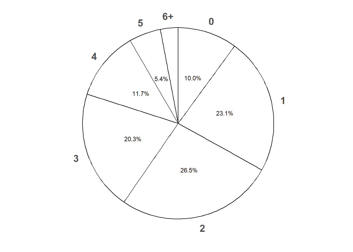
Example 14.3 Let $X$ be the number of home runs hit (in total by both teams) in a randomly selected Major League Baseball game. Technically, there is no fixed upper bound on what $X$ can be, so mathematically it is convenient to consider $0,1,2,\dots$ as the possible values of $X$. Assume that the pmf of $X$ is

$$p_X(x)=\{\begin{array}{ll}{e}^{-2.3}\frac{{2.3}^x}{x!},& x=0,1,2,\dots \\ 0,& \text{otherwise.}\end{array}$$

This is known as the Poisson(2.3) distribution.

1. Verify that $p_X$ is a valid pmf.
   
   
   
   
   

2. Compute $\text{P}(X=3)$, and interpret the value as a long run relative frequency.
   
   
   
   
   

3. Construct a table and spinner corresponding to the distribution of $X$.
   
   
   
   
   

4. Find $\text{P}(X\le 13)$, and interpret the value as a long run relative frequency. (The most home runs ever hit in a baseball game is 13.)
   
   
   
   
   

5. Use simulation to approximate the long run average value of $X$, and interpret this value.
   
   
   
   
   

6. Use simulation to approximate the variance and standard deviation of $X$.
   
   
   
   
   

• Poisson distributions are often used to model random variables that count “relatively rare events”.
• A discrete random variable $X$ has a Poisson distribution with parameter $\mu >0$ if its probability mass function $p_X$ satisfies $$p_X(x)=\frac{e^{-\mu }{\mu }^x}{x!},x=0,1,2,\dots$$
• The function ${\mu }^x/x!$ defines the shape of the pmf. The constant $e^{-\mu }$ ensures that the probabilities sum to 1.
• If $X$ has a Poisson($\mu$) distribution then $$\begin{array}{rl}\text{Long run average value of }X& =\mu \\ \text{Variance of }X& =\mu \\ \text{SD of }X& =\sqrt{\mu }\end{array}$$

Figure 14.1: Poisson(2.3) spinner

14.3 Binomial distributions

Example 14.4 Five messages of roughly equal length are to be transmitted across a noisy communication system. Assume the probability of any single message being transmitted successfully is 0.75, and that messages are transmitted independently of each other.

Let $X$ be the number of messages (out of 5) that are transmitted successfully.

1. Compute $\text{P}(X=0)$.
   
   
   
   
   

2. Compute the probability that the first message is transmitted successfully but the rest are not.
   
   
   
   
   

3. Compute $\text{P}(X=1)$.
   
   
   
   
   

4. Compute $\text{P}(X=2)$.
   
   
   
   
   

5. Find the pmf of $X$.
   
   
   
   
   

6. Construct a table, plot, and spinner representing the distribution of $X$.
   
   
   
   
   

7. Make an educated guess for the long run average value of $X$.
   
   
   
   
   

8. What does the random variable $Y=5-X$ measure? What is the distribution of $Y$?
   
   
   
   
   

• A discrete random variable $X$ has a Binomial distribution with parameters $n$, a nonnegative integer, and $p\in [0,1]$ if its probability mass function is $$\begin{array}{rlr}{p}_X(x)& =(\genfrac{}{}{0ex}{}{n}{x})p^x(1-p{)}^{n-x},& x=0,1,2,\dots ,n\end{array}$$
• If $X$ has a Binomial($n$, $p$) distribution then $$\begin{array}{rl}\text{Long run average value of }X& =np\\ \text{Variance of }X& =np(1-p)\\ \text{SD of }X& =\sqrt{np(1-p)}\end{array}$$
• Imagine a box containing tickets
  • With $p$ representing the proportion of tickets in the box labeled 1 (“success”); the rest are labeled 0 (“failure”).
  • Randomly select $n$ tickets from the box with replacement
  • Let $X$ be the number of tickets in the sample that are labeled 1.
  • Then $X$ has a Binomial($n$, $p$) distribution.
  • Since the tickets are labeled 1 and 0, the random variable $X$ which counts the number of successes is equal to the sum of the 1/0 values on the tickets.
  • If the selections are made with replacement, the draws are independent, so it is enough to just specify the population proportion $p$ without knowing the population size $N$.
• The situation in the previous bullets and the message example involves a sequence of Bernoulli trials.
  • There are only two possible outcomes, “success” (1) and “failure” (0), on each trial.
  • The unconditional/marginal probability of success is the same on every trial, and equal to $p$
  • The trials are independent.
• If $X$ counts the number of successes in a fixed number, $n$, of Bernoulli($p$) trials then $X$ has a Binomial($n,p$) distribution.

---

1. You can find a nice explanation of Benford’s law here.