Capítulo 15 Sistemas de Equacoes Lineares

Modelo $\mathbf{y_i} = \mathbf{ X_i \beta + u_i}$

onde: $y_i$ é Gx1, $X_i$ é GxK, $\beta$ é Kx1 e $u_i$ é Gx1.Sendo que $K = k_1 + ... + K_G$

15.0.1 SUR

Exemplo para dois indivíduos, 2 equações e 2 variáveis em cada equação

Nesse contexto $x$ possui três dimensões: $x_{ikg}$

$$\begin{bmatrix}y_{i1}\\ y_{i2} \end{bmatrix} = \begin{bmatrix}x_{i11} & x_{i21} & 0 & 0 \\ 0 & 0 & x_{i12} & x_{i22} \end{bmatrix} \begin{bmatrix} \beta_{11} \\ \beta_{21} \\ \beta_{12} \\ \beta_{22} \end{bmatrix} + \begin{bmatrix} u_{i1} \\ u_{i2} \end{bmatrix}$$

$$\begin{bmatrix}y_{i1}\\ y_{i2} \end{bmatrix} = \begin{bmatrix}x_{i11} \beta_{11} + x_{i21} \beta_{21} \\ x_{i12} \beta_{12} + x_{i22} \beta_{22} \end{bmatrix} + \begin{bmatrix} u_{i1} \\ u_{i2} \end{bmatrix}$$

Para uma Amostra N

$Y = X\beta + U$

onde: $Y$ é um vetor NGx1, $X$ uma matriz NGxK, $\beta$ um vetor Kx1 e $U$ um vetor NGx1.

Definir as variáveis explicativas do modelo

n = 1000
set.seed(1)
x1 = rnorm(n)
x2 = rnorm(n)

Definir os termos de erros, independentes porém correlacionados entre as equações.

library(mvtnorm)
sigma = matrix(c(4,3,3,30), ncol=2)
mv = rmvnorm(n, mean=c(0,0), sigma=sigma)
u1 = matrix(c(mv[,1]),ncol = 1)
u2 = matrix(c(mv[,2]),ncol = 1)
u = rbind(u1,u2)

Vetor $\beta$

beta1 = matrix(c(5,2,-1),ncol = 1)
beta2 = matrix(c(-5,-2,1),ncol = 1)
beta = rbind(beta1,beta2)

Organizando a matrix $X$

X1 = cbind(1,x1,x2)
X2 = cbind(1,x1,x2)
X = rbind(cbind(X1,0,0,0),cbind(0,0,0,X2))

Criando o vetor $Y$

Y = X%*%beta + u

Estimador SOLS

Sols = solve(t(X)%*%X)%*%t(X)%*%Y
Sols

##         [,1]
##     5.085939
## x1  1.979317
## x2 -1.104254
##    -5.068044
##    -2.089895
##     1.113130

Estimar Equação por Equação

y1 =  X1%*%beta1 + u1
y2 =  X2%*%beta2 + u2

ols1 = solve(t(X1)%*%X1)%*%t(X1)%*%y1
ols1

##         [,1]
##     5.085939
## x1  1.979317
## x2 -1.104254

ols2 = solve(t(X2)%*%X2)%*%t(X2)%*%y2
ols2

##         [,1]
##    -5.068044
## x1 -2.089895
## x2  1.113130

Matriz de Variância e Covariância

$\hat V(\hat\beta_{SOLS} = (X^{'}X)^{-1}X^{'}DX(X^{'}X)$

e_hat = Y - X%*%Sols
e = c(e_hat)
e = e * e
D = diag(e)
V_h = solve(t(X)%*%X)%*%(t(X)%*%D%*%X)%*%solve(t(X)%*%X)
V_h = (n/(n-6)) * V_h 
ep_h = sqrt(diag(V_h))
ep_h

##                    x1         x2                                  
## 0.06478291 0.05993167 0.06459487 0.18294688 0.17507186 0.17235189

e_hat1 = y1 - X1%*%ols1
e1 = c(e_hat1)
e1 = e1 * e1
D1 = diag(e1)
V_h1 = solve(t(X1)%*%X1)%*%(t(X1)%*%D1%*%X1)%*%solve(t(X1)%*%X1)
V_h1 = (n/(n-3)) * V_h1
ep_h1 = sqrt(diag(V_h1))
ep_h1

##                    x1         x2 
## 0.06468537 0.05984143 0.06449761

e_hat2 = y2 - X2%*%ols2
e2 = c(e_hat2)
e2 = e2 * e2
D2 = diag(e2)
V_h2 = solve(t(X2)%*%X2)%*%(t(X2)%*%D2%*%X2)%*%solve(t(X2)%*%X2)
V_h2 = (n/(n-3)) * V_h2
ep_h2 = sqrt(diag(V_h2))
ep_h2

##                  x1        x2 
## 0.1826714 0.1748083 0.1720924

15.1 FGLS

Estimar a matriz $\Omega = E(\mathbf u_i \mathbf u_i^{'})$.

$\hat\Omega = N^{-1} \sum_{i =1}^N u_i u_i^{'} = UU^{'}$

e_hat1 = y1 - X1%*%Sols[c(1,2,3),1]
e_hat2 = y2 - X2%*%Sols[c(4,5,6),1]
e_hat = cbind(e_hat1,e_hat2)

sigma = t(e_hat)%*%e_hat

$S = (I_N \otimes \Omega^{-1})$

I = diag(n)
S = kronecker(I,solve(sigma))   ## Wooldridge

$\hat\beta_{Fgls} = [X^{'}(\Omega^{-1} \otimes I_N)X]^{-1} [X^{'}(\Omega^{-1} \otimes I_N)Y]$

Bfgls = solve(t(X)%*%(S)%*%X)%*%(t(X)%*%(S)%*%Y)  ## Wooldridge
Bfgls

##         [,1]
##     4.982906
## x1  1.938422
## x2 -1.129926
##    -5.211998
##    -2.191069
##     1.046103

V =  solve(t(X)%*%S%*%X)%*%(t(X)%*%S%*%D%*%S%*%X)%*%solve(t(X)%*%S%*%X)
V = (1/(n-6)) * V
ep = sqrt(diag(V))
ep

##                      x1          x2                                     
## 0.002822832 0.002279409 0.002360631 0.007680877 0.006445076 0.006601576

$\hat V(\hat\beta_{Fgls}) = N^{-1} (X^{'}(\Omega^{-1} \otimes I_N)X)$

V_h = solve(t(X)%*%(S)%*%X)
V_h = (1/(n-6)) * V_h
ep_h = sqrt(diag(V_h))
ep_h

##                    x1         x2                                  
## 0.09158073 0.07939336 0.07606356 0.09158073 0.07939336 0.07606356

15.1.0.1 PAINEL

$$\begin{bmatrix}y_{i1}\\ y_{i2} \end{bmatrix} = \begin{bmatrix}x_{i11} & x_{i21} \\ x_{i12} & x_{i22} \end{bmatrix} \begin{bmatrix} \beta_{1} \\ \beta_{2} \end{bmatrix} + \begin{bmatrix} u_{i1} \\ u_{i2} \end{bmatrix}$$

n = 1000
set.seed(1)
x1 = rnorm(n)
x2 = rnorm(n)

sigma = matrix(c(4,3,3,30), ncol=2)
mv = rmvnorm(n, mean=c(0,0), sigma=sigma)
u1 = matrix(c(mv[,1]),ncol = 1)
u2 = matrix(c(mv[,2]),ncol = 1)
u = rbind(u1,u2)

beta = matrix(c(5,2,-1),ncol = 1)

X1 = cbind(1,x1,x2)
X2 = cbind(1,x1,x2)

y1 =  X1%*%beta + u1
y2 =  X2%*%beta + u2

X = rbind(X1,X2)

Y = X%*%beta + u

Pooled OLS

Pols = solve(t(X)%*%X)%*%t(X)%*%Y
Pols

##          [,1]
##     5.0089472
## x1  1.9447113
## x2 -0.9955618

e_hat = Y - X%*%Pols
e = c(e_hat)
e = e * e
D = diag(e)
V_h = solve(t(X)%*%X)%*%(t(X)%*%D%*%X)%*%solve(t(X)%*%X)
V_h = (n/(n-3)) * V_h  
ep_h = sqrt(diag(V_h))
ep_h

##                    x1         x2 
## 0.09694305 0.09244921 0.09192699

FGLS

e_hat1 = y1 - X1%*%Pols

e_hat2 = y2 - X2%*%Pols

e_hat = cbind(e_hat1,e_hat2)

sigma = t(e_hat)%*%e_hat
I = diag(n)
S = kronecker(I,solve(sigma))   ## Wooldridge

Bfgls = solve(t(X)%*%(S)%*%X)%*%(t(X)%*%(S)%*%Y)  ## Wooldridge
Bfgls

##         [,1]
##     4.885780
## x1  1.873816
## x2 -1.041929

V_h = solve(t(X)%*%(S)%*%X)
V_h = (1/(n)) * V_h
ep_h = sqrt(diag(V_h))
ep_h

##                    x1         x2 
## 0.06470610 0.05614001 0.05378698

15.2 Sistema de Equações com Variávies Instrumentais

15.2.1 2SLS

n = 1000
set.seed(1)
# Create independent variables
z1 = rnorm(n)
z2 = rnorm(n)

# Create error
u1 = rnorm(n)
u2 = rnorm(n)

# Create endogenous variable
x1 = .5*z1  -   z2 + u1 + rnorm(n)
x2 = 1.5*z1 - 2*z2 - u2 + rnorm(n)
x3 = rnorm(n)

# Create dependent variable
y1 =  5 + 2*x1 - x2 +   x3 + u1*5 - u2*2
y2 = -5 - 2*x1 + x2 - 2*x3 + u2*5 - u1*1
#X = cbind(x1,x2,x3,1)
#Y = cbind(y1,y2)

X = rbind(cbind(1,x1,x2,x3,0,0,0,0),cbind(0,0,0,0,1,x1,x2,x3))

Z = rbind(cbind(1,x3,z1,z2,0,0,0,0),cbind(0,0,0,0,1,x3,z1,z2))
Y = matrix(c(y1,y2),ncol=1)

Estimar por SOLS

Sols = solve(t(X)%*%X)%*%t(X)%*%Y
Sols

##          [,1]
##     5.0262660
## x1  3.8164234
## x2 -1.2994949
## x3  0.8788473
##    -4.9438961
##    -1.5682791
##     0.1883747
##    -1.9464426

sols = function(n){
   # Create independent variables
  z1 = rnorm(n)
  z2 = rnorm(n)
  # Create error
  u1 = rnorm(n)
  u2 = rnorm(n)
  # Create endogenous variable
  x1 = .5*z1  -   z2 + u1 + rnorm(n)
  x2 = 1.5*z1 - 2*z2 - u2 + rnorm(n)
  x3 = rnorm(n)
  # Create dependent variable
  y1 =  5 + 2*x1 - x2 +   x3 + u1*5 - u2*2
  y2 = -5 - 2*x1 + x2 - 2*x3 + u2*5 - u1*1
  X = rbind(cbind(1,x1,x2,x3,0,0,0,0),cbind(0,0,0,0,1,x1,x2,x3))
  Z = rbind(cbind(1,x3,z1,z2,0,0,0,0),cbind(0,0,0,0,1,x3,z1,z2))
  Y = matrix(c(y1,y2),ncol=1)  
  Sols = solve(t(X)%*%X)%*%t(X)%*%Y
  Sols
}
z = replicate(10000, expr = sols(1000))
par(mfrow = c(2, 2))

plot(density(z[2, 1, ]), xlim = c(0,4))
abline(v = 2)

plot(density(z[3, 1, ]), xlim = c(-2,0))
abline(v = -1)


plot(density(z[6, 1, ]), xlim = c(-4,0))
abline(v = -2)

plot(density(z[7, 1, ]), xlim = c(0,2))
abline(v = 1)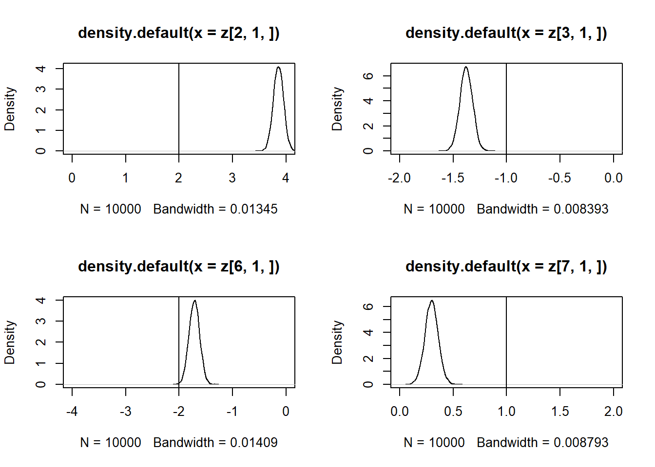

$\hat\beta(2sls) = [X^{'}Z(Z^{'}Z)^{-1}Z^{'}X]^{-1}$

SIV = solve(t(X)%*%Z%*%solve(t(Z)%*%Z)%*%t(Z)%*%X)%*%t(X)%*%Z%*%solve(t(Z)%*%Z)%*%t(Z)%*%Y
SIV

##          [,1]
##     5.0540920
## x1  0.6846211
## x2 -0.4035435
## x3  0.7844303
##    -4.9229999
##    -2.5418566
##     1.2379796
##    -1.8822475

sols = function(n){
   # Create independent variables
  z1 = rnorm(n)
  z2 = rnorm(n)
  # Create error
  u1 = rnorm(n)
  u2 = rnorm(n)
  # Create endogenous variable
  x1 = .5*z1  -   z2 + u1 + rnorm(n)
  x2 = 1.5*z1 - 2*z2 - u2 + rnorm(n)
  x3 = rnorm(n)
  # Create dependent variable
  y1 =  5 + 2*x1 - x2 +   x3 + u1*5 - u2*2
  y2 = -5 - 2*x1 + x2 - 2*x3 + u2*5 - u1*1
  X = rbind(cbind(1,x1,x2,x3,0,0,0,0),cbind(0,0,0,0,1,x1,x2,x3))
  Z = rbind(cbind(1,x3,z1,z2,0,0,0,0),cbind(0,0,0,0,1,x3,z1,z2))
  Y = matrix(c(y1,y2),ncol=1)  
  SIV = solve(t(X)%*%Z%*%solve(t(Z)%*%Z)%*%t(Z)%*%X)%*%t(X)%*%Z%*%solve(t(Z)%*%Z)%*%t(Z)%*%Y
  SIV
}
z = replicate(10000, expr = sols(1000))
par(mfrow = c(2, 2))

plot(density(z[2, 1, ]), xlim = c(0,4))
abline(v = 2)

plot(density(z[3, 1, ]), xlim = c(-2,0))
abline(v = -1)


plot(density(z[6, 1, ]), xlim = c(-4,0))
abline(v = -2)

plot(density(z[7, 1, ]), xlim = c(0,2))
abline(v = 1)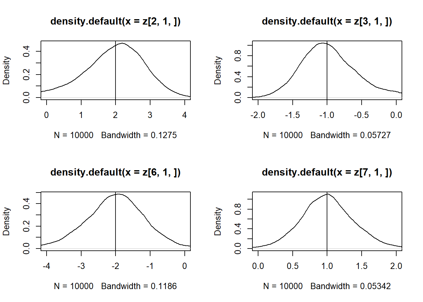

e_hat = Y - X%*%SIV
e = c(e_hat)
e = e * e
D = diag(e)
V_h = solve(t(X)%*%X)%*%(t(X)%*%D%*%X)%*%solve(t(X)%*%X)
V_h = (n/(n-8)) * V_h  ## Para comparar com a estimação equação por equação usa-se k = 4
ep_h = sqrt(diag(V_h))
ep_h

##                    x1         x2         x3                                  
## 0.21240194 0.20748985 0.09645245 0.20761424 0.17464545 0.12252813 0.08269950 
##            
## 0.17908589

Equção por equação

X = cbind(1,x1, x2, x3)
Y = cbind(y1,y2)
Z = cbind(1,x3, z1, z2)

IV1 = solve(t(X)%*%Z%*%solve(t(Z)%*%Z)%*%t(Z)%*%X)%*%t(X)%*%Z%*%solve(t(Z)%*%Z)%*%t(Z)%*%y1
IV1

##          [,1]
##     5.0540920
## x1  0.6846211
## x2 -0.4035435
## x3  0.7844303

IV2 = solve(t(X)%*%Z%*%solve(t(Z)%*%Z)%*%t(Z)%*%X)%*%t(X)%*%Z%*%solve(t(Z)%*%Z)%*%t(Z)%*%y2
IV2

##         [,1]
##    -4.923000
## x1 -2.541857
## x2  1.237980
## x3 -1.882247

15.2.2 FGLS - 3SLS

X1 = cbind(1,x1,x2,x3)
X2 = cbind(1,x1,x2,x3)

X = rbind(cbind(1,x1,x2,x3,0,0,0,0),cbind(0,0,0,0,1,x1,x2,x3))

Z = rbind(cbind(1,x3,z1,z2,0,0,0,0),cbind(0,0,0,0,1,x3,z1,z2))
Y = matrix(c(y1,y2),ncol=1)

e_hat1 = y1 - X1%*%SIV[c(1,2,3,4),1]
e_hat2 = y2 - X2%*%SIV[c(5,6,7,8),1]
e_hat = cbind(e_hat1,e_hat2)

sigma = t(e_hat)%*%e_hat
I = diag(n)
S1 = kronecker(I,solve(sigma)) 

Bfgls1 = solve(t(X)%*%Z%*%solve(t(Z)%*%S1%*%Z)%*%t(Z)%*%X)%*%t(X)%*%Z%*%solve(t(Z)%*%S1%*%Z)%*%t(Z)%*%Y
Bfgls1

##          [,1]
##     5.0540920
## x1  0.6846211
## x2 -0.4035435
## x3  0.7844303
##    -4.9229999
##    -2.5418566
##     1.2379796
##    -1.8822475

S2 = kronecker(I,sigma)

V_h = solve(t(X)%*%Z%*%solve(t(Z)%*%S2%*%Z)%*%t(Z)%*%X)
V_h = (1/(n)) * V_h
ep_h = sqrt(diag(V_h))
ep_h

##                  x1        x2        x3                                         
## 0.1669931 1.1803355 0.5236078 0.1840325 0.1669931 1.1803355 0.5236078 0.1840325