Documento 10 Iris dataset

1 - Cargamos los paquetes necesarios, además del dataset Iris.

library(rmarkdown)
library(knitr)
library(arules)
library(dplyr)
library(kableExtra)

data("iris")

A continuación, mostramos las 10 primeras filas del dataset a modo de ejemplo de visualización inicial:

kable(iris[1:10, ]) %>%
  kable_styling(bootstrap_options = c("striped", "hover", 
                                      "condensed"))

Sepal.Length	Sepal.Width	Petal.Length	Petal.Width	Species
5.1	3.5	1.4	0.2	setosa
4.9	3.0	1.4	0.2	setosa
4.7	3.2	1.3	0.2	setosa
4.6	3.1	1.5	0.2	setosa
5.0	3.6	1.4	0.2	setosa
5.4	3.9	1.7	0.4	setosa
4.6	3.4	1.4	0.3	setosa
5.0	3.4	1.5	0.2	setosa
4.4	2.9	1.4	0.2	setosa
4.9	3.1	1.5	0.1	setosa

2 - Utilizar las funciones que se han visto para analizar el dataset, ver número de transacciones, items del dataset, información estadística del dataset. NOTA: dataset debe ser preprocesado.

Con el comando str vemos la estructura de nuestro dataset, además del número de variables, tipo de dichas variables y sus primeros valores.

NOTA: Información antes del preprocesado.

str(iris)

'data.frame':   150 obs. of  5 variables:
 $ Sepal.Length: num  5.1 4.9 4.7 4.6 5 5.4 4.6 5 4.4 4.9 ...
 $ Sepal.Width : num  3.5 3 3.2 3.1 3.6 3.9 3.4 3.4 2.9 3.1 ...
 $ Petal.Length: num  1.4 1.4 1.3 1.5 1.4 1.7 1.4 1.5 1.4 1.5 ...
 $ Petal.Width : num  0.2 0.2 0.2 0.2 0.2 0.4 0.3 0.2 0.2 0.1 ...
 $ Species     : Factor w/ 3 levels "setosa","versicolor",..: 1 1 1 1 1 1 1 1 1 1 ...

Aquí vamos a comprobar la dimensión de nuestro dataset y, posteriormente, ver si se encuentra algún NA para eliminarlo del dataset.

# Número de filas y columnas
dim(iris)

[1] 150   5

# Comprobación de datos faltantes
sum(is.na(iris))

[1] 0

Con el comando summary obtenemos la información estadística pedida: mínimos, máximos, medias, etc de las variables de nuestro dataset.

summary(iris)

  Sepal.Length    Sepal.Width     Petal.Length    Petal.Width   
 Min.   :4.300   Min.   :2.000   Min.   :1.000   Min.   :0.100  
 1st Qu.:5.100   1st Qu.:2.800   1st Qu.:1.600   1st Qu.:0.300  
 Median :5.800   Median :3.000   Median :4.350   Median :1.300  
 Mean   :5.843   Mean   :3.057   Mean   :3.758   Mean   :1.199  
 3rd Qu.:6.400   3rd Qu.:3.300   3rd Qu.:5.100   3rd Qu.:1.800  
 Max.   :7.900   Max.   :4.400   Max.   :6.900   Max.   :2.500  
       Species  
 setosa    :50  
 versicolor:50  
 virginica :50

Discretizar de tres formas, guardando los resultados en tres datasets.

2.a) Transformando el tipo de las variables (convirtiendo a factor).

# Como vemos en str, sólo la variable "Species" es de tipo factor, 
# convertimos las demás:

dsIris1 <- iris

dsIris1$Sepal.Length <- ordered(cut(dsIris1$Sepal.Length, c(0, 5.4, 6.3, Inf)), labels = c("SL_Short", "SL_Medium", "SL_Large"))

#b1 <- c(4.3, 5.4, 6.3, 7.9)
#dsIris1$Sepal.Length <- cut(iris$Sepal.Length, breaks = b1, include.lowest = TRUE)

dsIris1$Sepal.Width <- ordered(cut(dsIris1$Sepal.Width, c(0, 2.9, 3.2, Inf)), labels = c("SW_Short", "SW_Medium", "SW_Large"))

#b2 <- c(2, 2.9, 3.2, 4.4)
#dsIris1$Sepal.Width <- cut(iris$Sepal.Width, breaks = b2, include.lowest = TRUE)

dsIris1$Petal.Length <- ordered(cut(dsIris1$Petal.Length, c(0, 2.63, 4.9, Inf)), labels = c("PL_Short", "PL_Medium", "PL_Large"))

#b3 <- c(1, 2.63, 4.9, 6.9)
#dsIris1$Petal.Length <- cut(iris$Petal.Length, breaks = b3, include.lowest = TRUE)

dsIris1$Petal.Width <- ordered(cut(dsIris1$Petal.Width, c(0, 0.867, 1.6, Inf)), labels = c("PW_Short", "PW_Medium", "PW_Large"))

#b4 <- c(0.1, 0.867, 1.6, 2.5)
#dsIris1$Petal.Width <- cut(iris$Petal.Width, breaks = b4, include.lowest = TRUE)

A continuación, mostramos cómo ha cambiado el dataset actual (dsIris1) del original mostrando de nuevo las 10 primeras filas:

kable(dsIris1[1:10, ]) %>%
  kable_styling(bootstrap_options = c("striped", "hover", 
                                      "condensed"))

Sepal.Length	Sepal.Width	Petal.Length	Petal.Width	Species
SL_Short	SW_Large	PL_Short	PW_Short	setosa
SL_Short	SW_Medium	PL_Short	PW_Short	setosa
SL_Short	SW_Medium	PL_Short	PW_Short	setosa
SL_Short	SW_Medium	PL_Short	PW_Short	setosa
SL_Short	SW_Large	PL_Short	PW_Short	setosa
SL_Short	SW_Large	PL_Short	PW_Short	setosa
SL_Short	SW_Large	PL_Short	PW_Short	setosa
SL_Short	SW_Large	PL_Short	PW_Short	setosa
SL_Short	SW_Short	PL_Short	PW_Short	setosa
SL_Short	SW_Medium	PL_Short	PW_Short	setosa

2.b) Discretizando los datos (convirtiendo en categóricos)

Creamos la variable en la que guardaremos el nuevo dataset

dsIris2 <- iris

Cambiamos el valor de los campos del nuevo dataset:

# Sepal.Length
dsIris2$Sepal.Length[dsIris2$Sepal.Length <= 5.4] <- "[4.3,5.4]"
dsIris2$Sepal.Length[dsIris2$Sepal.Length > 5.4  
                  & dsIris2$Sepal.Length <= 6.3] <- "(5.4, 6.3]"
dsIris2$Sepal.Length[dsIris2$Sepal.Length > 5.4] <- "(6.3,7.9]"

# Sepal.Width
dsIris2$Sepal.Width[dsIris2$Sepal.Width <= 2.9] <- "[2, 2.9]"
dsIris2$Sepal.Width[dsIris2$Sepal.Width > 2.9  
                  & dsIris2$Sepal.Width <= 3.2] <- "(2.9, 3.2]"
dsIris2$Sepal.Width[dsIris2$Sepal.Width > 3.2] <- "(3.2, 4.4]"

#Petal.Length
dsIris2$Petal.Length[dsIris2$Petal.Length <= 2.63] <- "[1, 2.63]"
dsIris2$Petal.Length[dsIris2$Petal.Length > 2.63  
                  & dsIris2$Petal.Length <= 4.9] <- "(2.63, 4.9]"
dsIris2$Petal.Length[dsIris2$Petal.Length > 4.9] <- "(4.9, 6.9]"

dsIris2$Petal.Width[dsIris2$Petal.Width <= 0.867] <- "[0.1, 0.867]"
dsIris2$Petal.Width[dsIris2$Petal.Width > 0.867  
                  & dsIris2$Petal.Width <= 1.6] <- "(0.867, 1.6]"
dsIris2$Petal.Width[dsIris2$Petal.Width > 1.6] <- "(1.6, 2.5]"

Convertimos los valores de tipo character en factor, creando 3 posibles valores (levels) de cada una de las variables.

dsIris2$Sepal.Length <- as.factor(dsIris2$Sepal.Length)
dsIris2$Sepal.Width <- as.factor(dsIris2$Sepal.Width)
dsIris2$Petal.Length <- as.factor(dsIris2$Petal.Length)
dsIris2$Petal.Width <- as.factor(dsIris2$Petal.Width)

A continuación, mostramos cómo ha cambiado el dataset actual (dsIris2) del original mostrando de nuevo las 10 primeras filas:

kable(dsIris2[1:10, ]) %>%
  kable_styling(bootstrap_options = c("striped", "hover", 
                                      "condensed"))

Sepal.Length	Sepal.Width	Petal.Length	Petal.Width	Species
[4.3,5.4]	(3.2, 4.4]	[1, 2.63]	[0.1, 0.867]	setosa
[4.3,5.4]	(2.9, 3.2]	[1, 2.63]	[0.1, 0.867]	setosa
[4.3,5.4]	(2.9, 3.2]	[1, 2.63]	[0.1, 0.867]	setosa
[4.3,5.4]	(2.9, 3.2]	[1, 2.63]	[0.1, 0.867]	setosa
[4.3,5.4]	(3.2, 4.4]	[1, 2.63]	[0.1, 0.867]	setosa
[4.3,5.4]	(3.2, 4.4]	[1, 2.63]	[0.1, 0.867]	setosa
[4.3,5.4]	(3.2, 4.4]	[1, 2.63]	[0.1, 0.867]	setosa
[4.3,5.4]	(3.2, 4.4]	[1, 2.63]	[0.1, 0.867]	setosa
[4.3,5.4]	[2, 2.9]	[1, 2.63]	[0.1, 0.867]	setosa
[4.3,5.4]	(2.9, 3.2]	[1, 2.63]	[0.1, 0.867]	setosa

2.c) Usando el comando discretize.

Para cada uno de los valores que no son de tipo factor, aplicamos el comando discretize para discretizar dichos valores.

dsIris3 <- iris

dsIris3$Sepal.Length <- discretize(iris$Sepal.Length, 
                            labels = c("SL_short", "SL_medium", "SL_long"),
                            method = "frequency", breaks = 3)

dsIris3$Sepal.Width <- discretize(iris$Sepal.Width, 
                            labels = c("SW_short", "SW_medium", "SW_long"),
                            method = "frequency", breaks = 3)

dsIris3$Petal.Length <- discretize(iris$Petal.Length, 
                            labels = c("PL_short", "PL_medium", "PL_long"),
                            method = "frequency", breaks = 3)

dsIris3$Petal.Width <- discretize(iris$Petal.Width, 
                            labels = c("PW_short", "PW_medium", "PW_long"),
                            method = "frequency", breaks = 3)

A continuación, mostramos cómo ha cambiado el dataset actual (dsIris3) del original mostrando de nuevo las 10 primeras filas:

kable(dsIris3[1:10, ]) %>%
  kable_styling(bootstrap_options = c("striped", "hover", 
                                      "condensed"))

Sepal.Length	Sepal.Width	Petal.Length	Petal.Width	Species
SL_short	SW_long	PL_short	PW_short	setosa
SL_short	SW_medium	PL_short	PW_short	setosa
SL_short	SW_long	PL_short	PW_short	setosa
SL_short	SW_medium	PL_short	PW_short	setosa
SL_short	SW_long	PL_short	PW_short	setosa
SL_medium	SW_long	PL_short	PW_short	setosa
SL_short	SW_long	PL_short	PW_short	setosa
SL_short	SW_long	PL_short	PW_short	setosa
SL_short	SW_medium	PL_short	PW_short	setosa
SL_short	SW_medium	PL_short	PW_short	setosa

Por último, convertimos los datasets a transacciones:

dsIris1 <- as(dsIris1, "transactions")
dsIris2 <- as(dsIris2, "transactions")
dsIris3 <- as(dsIris3, "transactions")
dsIris3

## transactions in sparse format with
##  150 transactions (rows) and
##  15 items (columns)

Vemos su estructura:

str(dsIris3)

Formal class 'transactions' [package "arules"] with 3 slots
  ..@ data       :Formal class 'ngCMatrix' [package "Matrix"] with 5 slots
  .. .. ..@ i       : int [1:750] 0 5 6 9 12 0 4 6 9 12 ...
  .. .. ..@ p       : int [1:151] 0 5 10 15 20 25 30 35 40 45 ...
  .. .. ..@ Dim     : int [1:2] 15 150
  .. .. ..@ Dimnames:List of 2
  .. .. .. ..$ : NULL
  .. .. .. ..$ : NULL
  .. .. ..@ factors : list()
  ..@ itemInfo   :'data.frame': 15 obs. of  3 variables:
  .. ..$ labels   : chr [1:15] "Sepal.Length=SL_short" "Sepal.Length=SL_medium" "Sepal.Length=SL_long" "Sepal.Width=SW_short" ...
  .. ..$ variables: Factor w/ 5 levels "Petal.Length",..: 3 3 3 4 4 4 1 1 1 2 ...
  .. ..$ levels   : Factor w/ 15 levels "PL_long","PL_medium",..: 10 9 8 13 12 11 3 2 1 6 ...
  ..@ itemsetInfo:'data.frame': 150 obs. of  1 variable:
  .. ..$ transactionID: chr [1:150] "1" "2" "3" "4" ...

Información estadística:

summary(dsIris3)

transactions as itemMatrix in sparse format with
 150 rows (elements/itemsets/transactions) and
 15 columns (items) and a density of 0.3333333 

most frequent items:
   Sepal.Width=SW_long Sepal.Length=SL_medium    Petal.Width=PW_long 
                    56                     53                     52 
  Sepal.Length=SL_long   Petal.Length=PL_long                (Other) 
                    51                     51                    487 

element (itemset/transaction) length distribution:
sizes
  5 
150 

   Min. 1st Qu.  Median    Mean 3rd Qu.    Max. 
      5       5       5       5       5       5 

includes extended item information - examples:
                  labels    variables    levels
1  Sepal.Length=SL_short Sepal.Length  SL_short
2 Sepal.Length=SL_medium Sepal.Length SL_medium
3   Sepal.Length=SL_long Sepal.Length   SL_long

includes extended transaction information - examples:
  transactionID
1             1
2             2
3             3

Por último, inspeccionamos las primeras filas (a modo de ejemplo):

inspect(dsIris3[1:2])

    items                   transactionID
[1] {Sepal.Length=SL_short,              
     Sepal.Width=SW_long,                
     Petal.Length=PL_short,              
     Petal.Width=PW_short,               
     Species=setosa}                    1
[2] {Sepal.Length=SL_short,              
     Sepal.Width=SW_medium,              
     Petal.Length=PL_short,              
     Petal.Width=PW_short,               
     Species=setosa}                    2

3 - Utilizar algoritmo apriori para obtener las reglas de asociación con confianza 0.5 y soporte 0.01. LLamar estas reglas r1.

r1 <- apriori(dsIris3,  parameter = list(supp = 0.01, conf = 0.5, target = "rules"))

Apriori

Parameter specification:
 confidence minval smax arem  aval originalSupport maxtime support minlen
        0.5    0.1    1 none FALSE            TRUE       5    0.01      1
 maxlen target   ext
     10  rules FALSE

Algorithmic control:
 filter tree heap memopt load sort verbose
    0.1 TRUE TRUE  FALSE TRUE    2    TRUE

Absolute minimum support count: 1 

set item appearances ...[0 item(s)] done [0.00s].
set transactions ...[15 item(s), 150 transaction(s)] done [0.00s].
sorting and recoding items ... [15 item(s)] done [0.00s].
creating transaction tree ... done [0.00s].
checking subsets of size 1 2 3 4 5 done [0.00s].
writing ... [532 rule(s)] done [0.00s].
creating S4 object  ... done [0.00s].

r1

set of 532 rules

4 - Encontrar reglas redundantes en r1 de dos formas distintas. Eliminarlas. Guardar en una variable las redundantes. Buscar en el paquete arules una función que te calcula las reglas redundantes.

Para empezar, definimos reglas redudantes como:

\(X => Y\) es redundante si existe un subset \(X’\) tal que: \(conf(X’ -> Y) >= conf(X -> Y)\)

Apunte: Una regla será redundante si existen reglas mas generales con la misma o mayor confianza, es decir, una regla más especifica es redundante si es igual o incluso menos predictiva que una regla más general.

FORMA 1:

# Guardando las reglas redundantes
idxRed <- which(is.redundant(r1))
vRed <- r1[idxRed]

# Guardando en r1 las reglas sin redundancia
idxNoRed <- which(!is.redundant(r1))
r1 <- r1[idxNoRed]
r1

## set of 196 rules

Si no queremos usar índices:

reglas_redundantes <- r1[is.redundant(r1)]
reglas_redundantes

## set of 0 rules

r1 <- r1[!is.redundant(r1)] #Quitamos las reglas redundantes
r1

## set of 196 rules

FORMA 2:

subset.matrix <- is.subset(r1, r1, sparse = FALSE)
subset.matrix[lower.tri(subset.matrix, diag = TRUE)] <- NA

reglas_redundantes2 <- colSums(subset.matrix, na.rm = TRUE) >= 1

length(which(reglas_redundantes2))

## [1] 163

reglas2 <- r1[!reglas_redundantes2] # 33
reglas2

## set of 33 rules

Con esta segunda forma obtenemos muchas menos reglas, obteniendo sólo un total de 33. Esta no es una versión muy eficiente de cómo sacar reglas redundantes y no se usa hoy en día.

5 - Generar 3 conjuntos de reglas que cumplan que ciertos valores estén a la izquierda y/o derecha. Llamarlas r2,r3,r4.

r2 <- apriori(dsIris3, 
              parameter = list(supp = 0.01, conf = 0.50),
              appearance = list(default="rhs",lhs="Sepal.Length=SL_medium"))

## Apriori
## 
## Parameter specification:
##  confidence minval smax arem  aval originalSupport maxtime support minlen
##         0.5    0.1    1 none FALSE            TRUE       5    0.01      1
##  maxlen target   ext
##      10  rules FALSE
## 
## Algorithmic control:
##  filter tree heap memopt load sort verbose
##     0.1 TRUE TRUE  FALSE TRUE    2    TRUE
## 
## Absolute minimum support count: 1 
## 
## set item appearances ...[1 item(s)] done [0.00s].
## set transactions ...[15 item(s), 150 transaction(s)] done [0.00s].
## sorting and recoding items ... [15 item(s)] done [0.00s].
## creating transaction tree ... done [0.00s].
## checking subsets of size 1 2 done [0.00s].
## writing ... [3 rule(s)] done [0.00s].
## creating S4 object  ... done [0.00s].

r3 <- apriori(dsIris3, 
              parameter = list(supp = 0.01, conf = 0.50),
              appearance = list(default = "lhs", rhs="Species=versicolor"))

## Apriori
## 
## Parameter specification:
##  confidence minval smax arem  aval originalSupport maxtime support minlen
##         0.5    0.1    1 none FALSE            TRUE       5    0.01      1
##  maxlen target   ext
##      10  rules FALSE
## 
## Algorithmic control:
##  filter tree heap memopt load sort verbose
##     0.1 TRUE TRUE  FALSE TRUE    2    TRUE
## 
## Absolute minimum support count: 1 
## 
## set item appearances ...[1 item(s)] done [0.00s].
## set transactions ...[15 item(s), 150 transaction(s)] done [0.00s].
## sorting and recoding items ... [15 item(s)] done [0.00s].
## creating transaction tree ... done [0.00s].
## checking subsets of size 1 2 3 4 5 done [0.00s].
## writing ... [51 rule(s)] done [0.00s].
## creating S4 object  ... done [0.00s].

r4 <- apriori(dsIris3, 
              parameter = list(supp = 0.01, conf = 0.50),
              appearance = list(rhs="Species=versicolor", lhs="Petal.Width=PW_medium"))

## Apriori
## 
## Parameter specification:
##  confidence minval smax arem  aval originalSupport maxtime support minlen
##         0.5    0.1    1 none FALSE            TRUE       5    0.01      1
##  maxlen target   ext
##      10  rules FALSE
## 
## Algorithmic control:
##  filter tree heap memopt load sort verbose
##     0.1 TRUE TRUE  FALSE TRUE    2    TRUE
## 
## Absolute minimum support count: 1 
## 
## set item appearances ...[2 item(s)] done [0.00s].
## set transactions ...[2 item(s), 150 transaction(s)] done [0.00s].
## sorting and recoding items ... [2 item(s)] done [0.00s].
## creating transaction tree ... done [0.00s].
## checking subsets of size 1 2 done [0.00s].
## writing ... [1 rule(s)] done [0.00s].
## creating S4 object  ... done [0.00s].

6 - Unir r2 y r3 y buscar reglas duplicadas y reglas redundantes.

rUnion <- c(r2,r3)  # 3 + 51
rUnion

## set of 54 rules

rUnion <- unique(rUnion)
rUnion

## set of 53 rules

Hay una regla repetida, la quitamos:

# Quitamos las reglas redundantes
rUnion <- rUnion[!is.redundant(rUnion)]
rUnion

## set of 18 rules

Otra forma (lapply):

rUnion <- lapply(c(r2,r3), unique)

Otra forma

rUnion <- union(r2,r3) # Quita las duplicadas directamente rUnion

7 - Hacer la intersección de r2 y r3.

Si queremos hallar la intersección de dos conjuntos de reglas basta con obtener los duplicados.

# Array de bool donde los TRUE son elementos duplicados
regs = c(r2,r3)
duplicados <- duplicated(regs)

# Obtenemos los índices de dichos elementos
elems <- which(duplicados)

# Guardamos en rInterseccion los elementos duplicados
rInterseccion <- regs[elems]
rInterseccion

## set of 1 rules

# ---- Otra forma

# rInterseccion <- intersect(r2,r3)
# rInterseccion

8 - Usa subset para inspeccionar las reglas con distintas condiciones.

1 - Selecciona todas las reglas con items “Species=setosa” o “Petal.Width=PW_medium” en la parte derecha y lift > 2

rules.sub_2 <- subset(r1, subset = rhs %in% c("Petal.Width=PW_medium","Species=setosa")&lift > 2)
inspect(rules.sub_2)

##      lhs                         rhs                        support confidence     lift count
## [1]  {Sepal.Length=SL_short}  => {Species=setosa}        0.26666667  0.8695652 2.608696    40
## [2]  {Petal.Length=PL_medium} => {Petal.Width=PW_medium} 0.28666667  0.8775510 2.742347    43
## [3]  {Species=versicolor}     => {Petal.Width=PW_medium} 0.30000000  0.9000000 2.812500    45
## [4]  {Petal.Length=PL_short}  => {Species=setosa}        0.33333333  1.0000000 3.000000    50
## [5]  {Petal.Width=PW_short}   => {Species=setosa}        0.33333333  1.0000000 3.000000    50
## [6]  {Sepal.Width=SW_long}    => {Species=setosa}        0.25333333  0.6785714 2.035714    38
## [7]  {Sepal.Length=SL_short,                                                                 
##       Sepal.Width=SW_medium}  => {Species=setosa}        0.07333333  1.0000000 3.000000    11
## [8]  {Sepal.Length=SL_short,                                                                 
##       Sepal.Width=SW_short}   => {Petal.Width=PW_medium} 0.03333333  0.7142857 2.232143     5
## [9]  {Sepal.Length=SL_short,                                                                 
##       Species=versicolor}     => {Petal.Width=PW_medium} 0.03333333  1.0000000 3.125000     5
## [10] {Sepal.Length=SL_short,                                                                 
##       Sepal.Width=SW_long}    => {Species=setosa}        0.18666667  1.0000000 3.000000    28
## [11] {Sepal.Width=SW_medium,                                                                 
##       Petal.Length=PL_medium} => {Petal.Width=PW_medium} 0.10666667  0.9411765 2.941176    16
## [12] {Sepal.Width=SW_medium,                                                                 
##       Species=versicolor}     => {Petal.Width=PW_medium} 0.11333333  0.9444444 2.951389    17
## [13] {Sepal.Length=SL_medium,                                                                
##       Sepal.Width=SW_medium}  => {Petal.Width=PW_medium} 0.07333333  0.7857143 2.455357    11
## [14] {Sepal.Width=SW_short,                                                                  
##       Petal.Length=PL_medium} => {Petal.Width=PW_medium} 0.16666667  0.9259259 2.893519    25
## [15] {Sepal.Width=SW_short,                                                                  
##       Species=versicolor}     => {Petal.Width=PW_medium} 0.17333333  0.9629630 3.009259    26
## [16] {Sepal.Length=SL_medium,                                                                
##       Sepal.Width=SW_short}   => {Petal.Width=PW_medium} 0.12666667  0.7307692 2.283654    19
## [17] {Petal.Length=PL_medium,                                                                
##       Species=versicolor}     => {Petal.Width=PW_medium} 0.28666667  0.9347826 2.921196    43
## [18] {Sepal.Length=SL_long,                                                                  
##       Petal.Length=PL_medium} => {Petal.Width=PW_medium} 0.06666667  0.9090909 2.840909    10
## [19] {Sepal.Length=SL_medium,                                                                
##       Species=versicolor}     => {Petal.Width=PW_medium} 0.18666667  0.9032258 2.822581    28
## [20] {Sepal.Length=SL_medium,                                                                
##       Sepal.Width=SW_long}    => {Species=setosa}        0.06666667  0.7692308 2.307692    10
## [21] {Sepal.Width=SW_medium,                                                                 
##       Petal.Length=PL_medium,                                                                
##       Species=versicolor}     => {Petal.Width=PW_medium} 0.10666667  1.0000000 3.125000    16
## [22] {Sepal.Length=SL_long,                                                                  
##       Sepal.Width=SW_medium,                                                                 
##       Petal.Length=PL_medium} => {Petal.Width=PW_medium} 0.03333333  1.0000000 3.125000     5
## [23] {Sepal.Length=SL_medium,                                                                
##       Sepal.Width=SW_medium,                                                                 
##       Species=versicolor}     => {Petal.Width=PW_medium} 0.07333333  1.0000000 3.125000    11
## [24] {Sepal.Width=SW_short,                                                                  
##       Petal.Length=PL_medium,                                                                
##       Species=versicolor}     => {Petal.Width=PW_medium} 0.16666667  1.0000000 3.125000    25
## [25] {Sepal.Length=SL_long,                                                                  
##       Sepal.Width=SW_short,                                                                  
##       Petal.Length=PL_medium} => {Petal.Width=PW_medium} 0.02000000  1.0000000 3.125000     3
## [26] {Sepal.Length=SL_medium,                                                                
##       Sepal.Width=SW_short,                                                                  
##       Petal.Length=PL_medium} => {Petal.Width=PW_medium} 0.11333333  0.9444444 2.951389    17
## [27] {Sepal.Length=SL_long,                                                                  
##       Sepal.Width=SW_short,                                                                  
##       Species=versicolor}     => {Petal.Width=PW_medium} 0.02666667  1.0000000 3.125000     4

2 - Selecciona solo las reglas con items “Species=setosa” y “Petal.Width=PW_medium” en la parte izquierda

rules.sub <- subset(r1, subset=lhs %ain% c("Species=versicolor", "Petal.Width=PW_medium"))
inspect(rules.sub)

##     lhs                         rhs                         support confidence     lift count
## [1] {Petal.Width=PW_medium,                                                                  
##      Species=versicolor}     => {Petal.Length=PL_medium} 0.28666667  0.9555556 2.925170    43
## [2] {Sepal.Width=SW_short,                                                                   
##      Petal.Width=PW_medium,                                                                  
##      Species=versicolor}     => {Petal.Length=PL_medium} 0.16666667  0.9615385 2.943485    25
## [3] {Sepal.Length=SL_medium,                                                                 
##      Petal.Width=PW_medium,                                                                  
##      Species=versicolor}     => {Petal.Length=PL_medium} 0.18666667  1.0000000 3.061224    28
## [4] {Petal.Length=PL_long,                                                                   
##      Petal.Width=PW_medium,                                                                  
##      Species=versicolor}     => {Sepal.Length=SL_long}   0.01333333  1.0000000 2.941176     2

3 - Usa coincidencia parcial para todos los item que se correspondan con la variable Species

rules.sub_3 <- subset(r1, subset = rhs %pin% "Species=")
inspect(rules.sub_3)

##      lhs                         rhs                     support confidence     lift count
## [1]  {Sepal.Length=SL_short}  => {Species=setosa}     0.26666667  0.8695652 2.608696    40
## [2]  {Sepal.Width=SW_short}   => {Species=versicolor} 0.18000000  0.5744681 1.723404    27
## [3]  {Petal.Width=PW_medium}  => {Species=versicolor} 0.30000000  0.9375000 2.812500    45
## [4]  {Petal.Length=PL_medium} => {Species=versicolor} 0.30666667  0.9387755 2.816327    46
## [5]  {Petal.Length=PL_short}  => {Species=setosa}     0.33333333  1.0000000 3.000000    50
## [6]  {Petal.Width=PW_short}   => {Species=setosa}     0.33333333  1.0000000 3.000000    50
## [7]  {Sepal.Width=SW_long}    => {Species=setosa}     0.25333333  0.6785714 2.035714    38
## [8]  {Sepal.Length=SL_medium} => {Species=versicolor} 0.20666667  0.5849057 1.754717    31
## [9]  {Sepal.Length=SL_long}   => {Species=virginica}  0.24666667  0.7254902 2.176471    37
## [10] {Petal.Length=PL_long}   => {Species=virginica}  0.31333333  0.9215686 2.764706    47
## [11] {Petal.Width=PW_long}    => {Species=virginica}  0.31333333  0.9038462 2.711538    47
## [12] {Sepal.Length=SL_short,                                                              
##       Sepal.Width=SW_medium}  => {Species=setosa}     0.07333333  1.0000000 3.000000    11
## [13] {Sepal.Length=SL_short,                                                              
##       Sepal.Width=SW_short}   => {Species=versicolor} 0.03333333  0.7142857 2.142857     5
## [14] {Sepal.Length=SL_short,                                                              
##       Petal.Width=PW_medium}  => {Species=versicolor} 0.03333333  1.0000000 3.000000     5
## [15] {Sepal.Length=SL_short,                                                              
##       Sepal.Width=SW_long}    => {Species=setosa}     0.18666667  1.0000000 3.000000    28
## [16] {Sepal.Width=SW_medium,                                                              
##       Petal.Width=PW_medium}  => {Species=versicolor} 0.11333333  1.0000000 3.000000    17
## [17] {Sepal.Width=SW_medium,                                                              
##       Petal.Length=PL_medium} => {Species=versicolor} 0.10666667  0.9411765 2.823529    16
## [18] {Sepal.Length=SL_medium,                                                             
##       Sepal.Width=SW_medium}  => {Species=versicolor} 0.07333333  0.7857143 2.357143    11
## [19] {Sepal.Width=SW_medium,                                                              
##       Petal.Width=PW_long}    => {Species=virginica}  0.12000000  0.9473684 2.842105    18
## [20] {Sepal.Length=SL_medium,                                                             
##       Sepal.Width=SW_short}   => {Species=versicolor} 0.12000000  0.6923077 2.076923    18
## [21] {Sepal.Width=SW_short,                                                               
##       Petal.Width=PW_long}    => {Species=virginica}  0.10666667  0.9411765 2.823529    16
## [22] {Petal.Length=PL_medium,                                                             
##       Petal.Width=PW_medium}  => {Species=versicolor} 0.28666667  1.0000000 3.000000    43
## [23] {Sepal.Width=SW_long,                                                                
##       Petal.Width=PW_medium}  => {Species=versicolor} 0.01333333  1.0000000 3.000000     2
## [24] {Sepal.Length=SL_long,                                                               
##       Petal.Length=PL_medium} => {Species=versicolor} 0.07333333  1.0000000 3.000000    11
## [25] {Sepal.Width=SW_long,                                                                
##       Petal.Length=PL_medium} => {Species=versicolor} 0.03333333  1.0000000 3.000000     5
## [26] {Sepal.Length=SL_medium,                                                             
##       Sepal.Width=SW_long}    => {Species=setosa}     0.06666667  0.7692308 2.307692    10
## [27] {Sepal.Length=SL_long,                                                               
##       Petal.Length=PL_long}   => {Species=virginica}  0.24666667  0.9250000 2.775000    37
## [28] {Sepal.Length=SL_long,                                                               
##       Petal.Width=PW_long}    => {Species=virginica}  0.24000000  0.9473684 2.842105    36
## [29] {Sepal.Length=SL_long,                                                               
##       Sepal.Width=SW_long}    => {Species=virginica}  0.08000000  0.8000000 2.400000    12
## [30] {Petal.Length=PL_long,                                                               
##       Petal.Width=PW_long}    => {Species=virginica}  0.29333333  0.9565217 2.869565    44
## [31] {Sepal.Width=SW_long,                                                                
##       Petal.Length=PL_long}   => {Species=virginica}  0.08666667  1.0000000 3.000000    13
## [32] {Sepal.Length=SL_medium,                                                             
##       Sepal.Width=SW_medium,                                                              
##       Petal.Length=PL_long}   => {Species=virginica}  0.01333333  1.0000000 3.000000     2
## [33] {Sepal.Length=SL_medium,                                                             
##       Sepal.Width=SW_medium,                                                              
##       Petal.Width=PW_long}    => {Species=virginica}  0.02000000  1.0000000 3.000000     3
## [34] {Sepal.Length=SL_medium,                                                             
##       Sepal.Width=SW_short,                                                               
##       Petal.Length=PL_medium} => {Species=versicolor} 0.11333333  0.9444444 2.833333    17
## [35] {Sepal.Width=SW_short,                                                               
##       Petal.Length=PL_medium,                                                             
##       Petal.Width=PW_long}    => {Species=virginica}  0.01333333  1.0000000 3.000000     2
## [36] {Sepal.Length=SL_long,                                                               
##       Sepal.Width=SW_short,                                                               
##       Petal.Width=PW_long}    => {Species=virginica}  0.06000000  1.0000000 3.000000     9
## [37] {Sepal.Length=SL_medium,                                                             
##       Petal.Length=PL_long,                                                               
##       Petal.Width=PW_medium}  => {Species=virginica}  0.01333333  1.0000000 3.000000     2
## [38] {Sepal.Length=SL_medium,                                                             
##       Sepal.Width=SW_long,                                                                
##       Petal.Width=PW_long}    => {Species=versicolor} 0.01333333  0.6666667 2.000000     2
## [39] {Sepal.Length=SL_long,                                                               
##       Petal.Length=PL_long,                                                               
##       Petal.Width=PW_long}    => {Species=virginica}  0.24000000  0.9729730 2.918919    36

Siendo:
- %in%: Selecciona conjuntos de elementos que coincidan con cualquier elemento dado.
- %ain%: Selecciona solo conjuntos de elementos que coincidan con todos los elementos dados.
- %oin%: Selecciona conjuntos de elementos que solo coincidan con el elemento dado.
- %pin%: %in% con ‘partial matching’.

9 - Usa summary, sort.

Summary: Devuelve una visión general del conjunto de reglas de asociación.

summary(r1)

## set of 196 rules
## 
## rule length distribution (lhs + rhs):sizes
##   2   3   4 
##  51 109  36 
## 
##    Min. 1st Qu.  Median    Mean 3rd Qu.    Max. 
##   2.000   2.000   3.000   2.923   3.000   4.000 
## 
## summary of quality measures:
##     support          confidence          lift           count      
##  Min.   :0.01333   Min.   :0.5000   Min.   :1.339   Min.   : 2.00  
##  1st Qu.:0.04000   1st Qu.:0.7025   1st Qu.:2.109   1st Qu.: 6.00  
##  Median :0.11333   Median :0.9208   Median :2.713   Median :17.00  
##  Mean   :0.13480   Mean   :0.8470   Mean   :2.542   Mean   :20.22  
##  3rd Qu.:0.24000   3rd Qu.:1.0000   3rd Qu.:2.951   3rd Qu.:36.00  
##  Max.   :0.33333   Max.   :1.0000   Max.   :3.261   Max.   :50.00  
## 
## mining info:
##     data ntransactions support confidence
##  dsIris3           150    0.01        0.5

Sort: Ordena los elementos dependiendo del valor de las variables pasadas por parámetro:

r1.ordenado <- sort(r1,  by = "support", decreasing = TRUE)

r1.ordenado

## set of 196 rules

10 - Explicar y usar los comandos de paquete arules siguientes: dissimilarity, image, is.redundant, is.significant, itemFrequency.

Dissimilarity: Utiliza la función de distancia para calcular estadísticas de disimilitud agrupando variables.

Disimilitud: Se corresponde con el cálculo de falta de semejanza entre dos objetos principalmente.

dissimilarity(r2)

##           1         2
## 2 0.6666667          
## 3 0.6666667 0.6666667

image: Genera gráficos “de nivel” para inspeccionar visualmente las matrices de incidencia binarias.

# Cogemos los primeros 50 elementos para que la imagen no 
# se vea tan sobrecargada
image(dsIris3[1:50])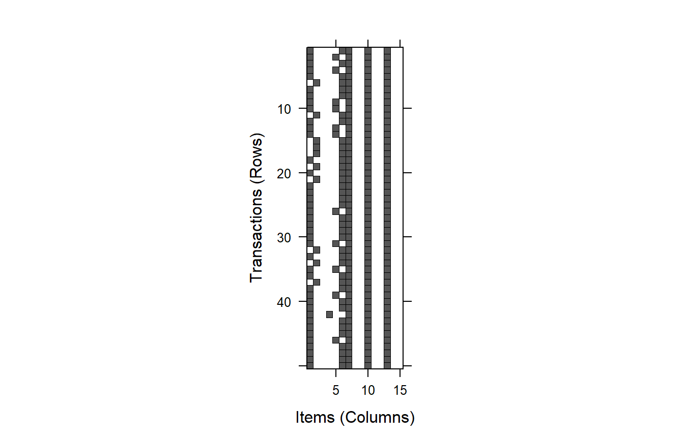

itemFrequency: devuelve la frecuencia de cada item.

frecuencia_items <- itemFrequency(items(r1))
frecuencia_items

##  Sepal.Length=SL_short Sepal.Length=SL_medium   Sepal.Length=SL_long 
##             0.13775510             0.28061224             0.21938776 
##   Sepal.Width=SW_short  Sepal.Width=SW_medium    Sepal.Width=SW_long 
##             0.22959184             0.19387755             0.22959184 
##  Petal.Length=PL_short Petal.Length=PL_medium   Petal.Length=PL_long 
##             0.06632653             0.28571429             0.19387755 
##   Petal.Width=PW_short  Petal.Width=PW_medium    Petal.Width=PW_long 
##             0.06632653             0.26530612             0.22959184 
##         Species=setosa     Species=versicolor      Species=virginica 
##             0.06632653             0.27040816             0.18877551

freqdsIris3 <- itemFrequency(dsIris3)
freqdsIris3

##  Sepal.Length=SL_short Sepal.Length=SL_medium   Sepal.Length=SL_long 
##              0.3066667              0.3533333              0.3400000 
##   Sepal.Width=SW_short  Sepal.Width=SW_medium    Sepal.Width=SW_long 
##              0.3133333              0.3133333              0.3733333 
##  Petal.Length=PL_short Petal.Length=PL_medium   Petal.Length=PL_long 
##              0.3333333              0.3266667              0.3400000 
##   Petal.Width=PW_short  Petal.Width=PW_medium    Petal.Width=PW_long 
##              0.3333333              0.3200000              0.3466667 
##         Species=setosa     Species=versicolor      Species=virginica 
##              0.3333333              0.3333333              0.3333333

is.redundant: Encuentra los elementos redudantes de un conjunto de reglas

Ejemplo ya visto en varias ocasiones a lo largo de la presentación.

is.significant: Encuentra reglas donde el LHS y el RHS dependen el uno del otro.

is.significant(r2, r3)

## [1] FALSE FALSE FALSE

En este caso vemos que no depende ninguna regla entre r2 y r3