Documento 21 Analisis de Tweets:
- Introduce tus claves en el documento para conectar con Twitter. Usa en el chunk la opción echo=FALSE, para no mostrar tus claves en el documento de salida.
NOTA: Los twits se extrajeron en Rstudio Cloud.
Nos autenticamos.
## authenticate via web browser
token <- create_token(
  app = "TwitsIgnacioPG",
  consumer_key = api_key,
  consumer_secret = api_secret_key,
  access_token = access_token,
  access_secret = access_token_secret)
Los tweets fueron extraídos con el siguiente comando:
Para posteriormente escribirlos en un .csv
- Paquetes necesarios:
library(rtweet)
library(httpuv)
library(readr)
library(lubridate)
library(tm)
library(wordcloud)
library(wordcloud2)
library(rmarkdown)
library(ggthemes)
library(ggplot2)
- Extraer de Twitter los tweets referentes a un tema que a ti te interese. Pasa los tweets a un dataframe y visualiza la cabeza del data frame. Graba los tweets en un csv.
## Warning: Missing column names filled in: 'X1' [1]## Parsed with column specification:
## cols(
## X1 = col_double(),
## text = col_character(),
## favorited = col_logical(),
## favoriteCount = col_double(),
## replyToSN = col_character(),
## created = col_datetime(format = ""),
## truncated = col_logical(),
## replyToSID = col_double(),
## id = col_double(),
## replyToUID = col_double(),
## statusSource = col_character(),
## screenName = col_character(),
## retweetCount = col_double(),
## isRetweet = col_logical(),
## retweeted = col_logical(),
## longitude = col_logical(),
## latitude = col_logical()
## )# Convierto a data frame el csv haciendo uso de la funcion glmpse de dplyr
pizzagate <- dplyr::glimpse(tweets)## Observations: 5,000
## Variables: 17
## $ X1 <dbl> 1, 2, 3, 4, 5, 6, 7, 8, 9, 10, 11, 12, 13, 14, 15, 16...
## $ text <chr> "RT @BenjaminCespe17: Take the red pill\nit's time to...
## $ favorited <lgl> FALSE, FALSE, FALSE, FALSE, FALSE, FALSE, FALSE, FALS...
## $ favoriteCount <dbl> 0, 0, 0, 0, 0, 0, 0, 0, 0, 0, 0, 0, 0, 0, 0, 0, 0, 0,...
## $ replyToSN <chr> NA, NA, NA, NA, "ClaudiaSilver7", NA, NA, NA, NA, NA,...
## $ created <dttm> 2020-06-01 08:03:19, 2020-06-01 08:03:18, 2020-06-01...
## $ truncated <lgl> FALSE, FALSE, FALSE, FALSE, TRUE, FALSE, FALSE, FALSE...
## $ replyToSID <dbl> NA, NA, NA, NA, 1.267352e+18, NA, NA, NA, NA, NA, NA,...
## $ id <dbl> 1.267366e+18, 1.267366e+18, 1.267366e+18, 1.267366e+1...
## $ replyToUID <dbl> NA, NA, NA, NA, 7.503714e+17, NA, NA, NA, NA, NA, NA,...
## $ statusSource <chr> "<a href=\"http://twitter.com/download/android\" rel=...
## $ screenName <chr> "Mikemoralitos1", "here5johnny", "Nerlux2", "EimyNami...
## $ retweetCount <dbl> 35, 105, 5, 53, 0, 53, 1295, 35, 5, 53, 2, 1295, 158,...
## $ isRetweet <lgl> TRUE, TRUE, TRUE, TRUE, FALSE, TRUE, TRUE, TRUE, TRUE...
## $ retweeted <lgl> FALSE, FALSE, FALSE, FALSE, FALSE, FALSE, FALSE, FALS...
## $ longitude <lgl> NA, NA, NA, NA, NA, NA, NA, NA, NA, NA, NA, NA, NA, N...
## $ latitude <lgl> NA, NA, NA, NA, NA, NA, NA, NA, NA, NA, NA, NA, NA, N...# Limpieza rápida del dataset
# tweets.df = twListToDF(tweets2) - Esta no es necesaria pues los tweets ya estan en formato df
pizzagate$text <- sapply(pizzagate$text,function(x) iconv(x,to='UTF-8'))
pizzagate$created <- ymd_hms(pizzagate$created)
# Comprobamos en que columnas hay valores NA
sapply(pizzagate, function(x) sum(is.na(x)))## X1 text favorited favoriteCount replyToSN
## 0 0 0 0 4742
## created truncated replyToSID id replyToUID
## 0 0 4757 0 4742
## statusSource screenName retweetCount isRetweet retweeted
## 0 0 0 0 0
## longitude latitude
## 5000 5000# Como en las columnas Latitude y Longitude sólo hay NAs, las eliminamos:
pizzagate$latitude <- NULL
pizzagate$longitude <- NULL
head(pizzagate)## # A tibble: 6 x 15
## X1 text favorited favoriteCount replyToSN created truncated
## <dbl> <chr> <lgl> <dbl> <chr> <dttm> <lgl>
## 1 1 "RT ~ FALSE 0 <NA> 2020-06-01 08:03:19 FALSE
## 2 2 "RT ~ FALSE 0 <NA> 2020-06-01 08:03:18 FALSE
## 3 3 "RT ~ FALSE 0 <NA> 2020-06-01 08:02:23 FALSE
## 4 4 "RT ~ FALSE 0 <NA> 2020-06-01 08:02:10 FALSE
## 5 5 "@Cl~ FALSE 0 ClaudiaS~ 2020-06-01 08:02:06 TRUE
## 6 6 "RT ~ FALSE 0 <NA> 2020-06-01 08:01:41 FALSE
## # ... with 8 more variables: replyToSID <dbl>, id <dbl>, replyToUID <dbl>,
## # statusSource <chr>, screenName <chr>, retweetCount <dbl>, isRetweet <lgl>,
## # retweeted <lgl>- ¿Cuantos tweets hay?
## [1] 5000- Analiza la estructura de la información que te has traido de Twitter.
## [1] "spec_tbl_df" "tbl_df" "tbl" "data.frame"## Classes 'spec_tbl_df', 'tbl_df', 'tbl' and 'data.frame': 5000 obs. of 15 variables:
## $ X1 : num 1 2 3 4 5 6 7 8 9 10 ...
## $ text : chr "RT @BenjaminCespe17: Take the red pill\nit's time to open your eyes.\n#anonymus #pizzagate \n#WhiteHouse https:"| __truncated__ "RT @cafemonera: #Anonymous right now after ignoring #PizzaGate, the arrest of Julian Assange and the release of"| __truncated__ "RT @Ealaguice: Itâ\200\231s not about the burn of a flag, itâ\200\231s about the downfall of the elite, lies an"| __truncated__ "RT @ItsOVER16274589: ðŸ‘\201ï¸\217â\200\215🗨ï¸\217\nDEMI MOORE\n13-years-old Childactor Philip Tanzini is ge"| __truncated__ ...
## $ favorited : logi FALSE FALSE FALSE FALSE FALSE FALSE ...
## $ favoriteCount: num 0 0 0 0 0 0 0 0 0 0 ...
## $ replyToSN : chr NA NA NA NA ...
## $ created : POSIXct, format: "2020-06-01 08:03:19" "2020-06-01 08:03:18" ...
## $ truncated : logi FALSE FALSE FALSE FALSE TRUE FALSE ...
## $ replyToSID : num NA NA NA NA 1.27e+18 ...
## $ id : num 1.27e+18 1.27e+18 1.27e+18 1.27e+18 1.27e+18 ...
## $ replyToUID : num NA NA NA NA 7.5e+17 ...
## $ statusSource : chr "<a href=\"http://twitter.com/download/android\" rel=\"nofollow\">Twitter for Android</a>" "<a href=\"https://mobile.twitter.com\" rel=\"nofollow\">Twitter Web App</a>" "<a href=\"https://mobile.twitter.com\" rel=\"nofollow\">Twitter Web App</a>" "<a href=\"https://mobile.twitter.com\" rel=\"nofollow\">Twitter Web App</a>" ...
## $ screenName : chr "Mikemoralitos1" "here5johnny" "Nerlux2" "EimyNamie" ...
## $ retweetCount : num 35 105 5 53 0 ...
## $ isRetweet : logi TRUE TRUE TRUE TRUE FALSE TRUE ...
## $ retweeted : logi FALSE FALSE FALSE FALSE FALSE FALSE ...
## - attr(*, "spec")=
## .. cols(
## .. X1 = col_double(),
## .. text = col_character(),
## .. favorited = col_logical(),
## .. favoriteCount = col_double(),
## .. replyToSN = col_character(),
## .. created = col_datetime(format = ""),
## .. truncated = col_logical(),
## .. replyToSID = col_double(),
## .. id = col_double(),
## .. replyToUID = col_double(),
## .. statusSource = col_character(),
## .. screenName = col_character(),
## .. retweetCount = col_double(),
## .. isRetweet = col_logical(),
## .. retweeted = col_logical(),
## .. longitude = col_logical(),
## .. latitude = col_logical()
## .. )Analizando las columnas más importantes:
X1: Parecido a una ID Text: Contenido del tweet ScreenName: Procedencia del tweet Created: Fecha de creación retweetCount: Número de rts favoriteCount: Número de favs isRetweet: Si el tweet original ha sido retweeteado
- ¿Cuantos usuarios distintos han participado?
## [1] 5000- ¿Cuantos tweets son re-tweets? (isRetweet)
## [1] 4290- ¿Cuantos tweets han sido re-tweeteados? (retweeted)
# Este campo nos dicen los rt que ha tenido un twit original, como la mayoría son twits retuiteados, y los originales no tienen ningún retweet

nrow(pizzagate[pizzagate$retweeted == TRUE, ])
## [1] 0- ¿Cuál es el número medio de retweets? (retweetCount)
## [1] 325.137- Da una lista con los distintos idiomas que se han usado al twitear este hashtag. (language).
No hemos podido conseguir esta información, pero al extraer todos los tweets pusimos en el parámetro de research que todos fueras en inglés.
- Encontrar los nombres de usuarios de las 10 personas que más han participado.
##     bananedave    RoRoFlores8 Aleszanderizsk     mystylehfb        DDemaos
##             28             28             21             21             20
##    LanceFahey1  Cindy67427591     FocusOutof         dgxpre       MtzrYadi
## 18 16 15 14 13- ¿Quién es el usuario que más ha participado?
## bananedave
## 28- Extraer en un data frame aquellos tweets re-tuiteados más de 5 veces (retweetCount).
# Primero eliminare los que son rt
indices <- which(!pizzagate$isRetweet)
pizzagateSinRt <- pizzagate[indices,]

famosos <- pizzagateSinRt %>%
  dplyr::filter(retweetCount >= 5) %>%
  dplyr::select(text, id, retweetCount)

famosos
## # A tibble: 56 x 3
## text id retweetCount
## <chr> <dbl> <dbl>
## 1 "Lady gaga and marina Abramovic ingesting the drug adre~ 1.27e18 5
## 2 "It’s not about the burn of a flag, it’s about the ~ 1.27e18 5
## 3 "Take the red pill\nit's time to open your eyes.\n#anon~ 1.27e18 35
## 4 "@BarbMcQuade Never forget, it was Wikileaks & the ~ 1.27e18 7
## 5 "THIS IS AMERICA!\n#Anonymous #JusticeForGeorgeFloyd #P~ 1.27e18 7
## 6 "#anonymus Casa Blanca #PizzaGate \nmy mood: https://t.~ 1.27e18 5
## 7 "#Anonymous #pizzagate #Trump\nI propose 'Panic' by The~ 1.27e18 16
## 8 "Do you remember this?\nI think it's time you are going~ 1.27e18 6
## 9 "OUTFIT MAYO / OUFIT JUNIO casa blanca trump anonymous ~ 1.27e18 24
## 10 "Casa Blanca, #anonymus #PizzaGate The Purge\nMaaaaaan,~ 1.27e18 7
## # ... with 46 more rows- Aplicarle a los tweets las técnicas de Text-Mining vistas en clase:
- Haz pre-procesamiento adecuado.
toSpace <- content_transformer(function(x, pattern) gsub(pattern, " ", x))
toString <- content_transformer(function(x, from, to) gsub(from, to, x))

pizzagate$text <- stringr::str_replace_all(pizzagate$text, "@\\w+"," ")
pizzagate$text <- stringr::str_replace_all(pizzagate$text, "#\\S+"," ")## Remove Hashtags
pizzagate$text <- stringr::str_replace_all(pizzagate$text, "http\\S+\\s*"," ")## Remove URLs
pizzagate$text <- stringr::str_replace_all(pizzagate$text, "http[[:alnum:]]*"," ")## Remove URLs
pizzagate$text <- stringr::str_replace_all(pizzagate$text, "http[[\\b+RT]]"," ")## Remove URLs
pizzagate$text <- stringr::str_replace_all(pizzagate$text, "[[:cntrl:]]"," ")
pizzagate$text <- stringr::str_replace_all(pizzagate$text, "#pizzagate"," ")

pizzagate$text <- stringr::str_replace_all(pizzagate$text, "[^\\x00-\\x7F]"," ")

docsCorpus <- Corpus(VectorSource(pizzagate$text))
docsCorpus <- tm_map(docsCorpus, function(x) iconv(enc2utf8(x), sub = "byte"))

Textprocessing <- function(x)
  {gsub("http[[:alnum:]]*",'', x)
  gsub('http\\S+\\s*', '', x) ## Remove URLs
  gsub('\\b+RT', '', x) ## Remove RT
  gsub('#\\S+', '', x) ## Remove Hashtags
  gsub('@\\S+', '', x) ## Remove Mentions
  gsub('[[:cntrl:]]', '', x) ## Remove Controls and special characters
  gsub("\\d", '', x) ## Remove Controls and special characters
  gsub('[[:punct:]]', '', x) ## Remove Punctuations
  gsub("^[[:space:]]*","",x) ## Remove leading whitespaces
  gsub("[[:space:]]*$","",x) ## Remove trailing whitespaces
  gsub(' +',' ',x) ## Remove extra whitespaces
}

docsCorpus <- tm_map(docsCorpus,Textprocessing)

docsCorpus <- tm_map(docsCorpus, content_transformer(tolower))

docsCorpus <- tm_map(docsCorpus, removeNumbers)

docsCorpus <- tm_map(docsCorpus, removePunctuation)

docsCorpus <- tm_map(docsCorpus, stripWhitespace)

docsCorpus <- tm_map(docsCorpus, removeWords, stopwords("english"))

docsCorpus <- tm_map(docsCorpus, toSpace, "rt")
Genero DTM
## <<DocumentTermMatrix (documents: 5000, terms: 2319)>>
## Non-/sparse entries: 41176/11553824
## Sparsity           : 100%
## Maximal term length: 29
## Weighting : term frequency (tf)- Calcula la media de la frecuencia de aparición de los términos.
- Encuentra los términos que ocurren más de la media y guárdalos en un data.frame: término y su frecuencia. Usa knitr::kable en el .Rmd siempre que quieras visualizar los data.frame.
- Ordena este data.frame por la frecuencia
##  enough   yummy    live actions  result  rioter
## 19 19 19 19 19 19## hollywood pedophilia exposing exposed star since
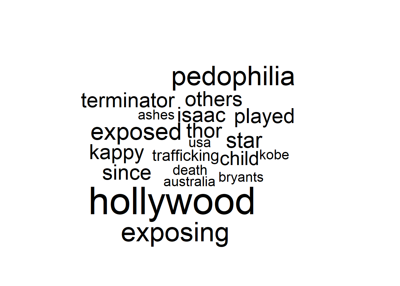
## 1348 901 898 785 683 660- Haz un plot de los términos más frecuentes. Si salen muchos términos visualiza un número adecuado de palabras para que se pueda ver algo.
set.seed(142)
# Distintas paletas de colores
# brewer.pal(6, "Dark2")
# brewer.pal(9,"YlGnBu")
#wordcloud(names(freq), freq, min.freq=350, max.words=50, scale=c(5, .1), colors=brewer.pal(6, "Dark2"))
#set.seed(42)
wordcloud(names(freq2), freq2, scale=c(3,0.5), max.words=60, random.order=FALSE,
rot.per=0.10, use.r.layout=TRUE, colors=brewer.pal(6, "Dark2")) 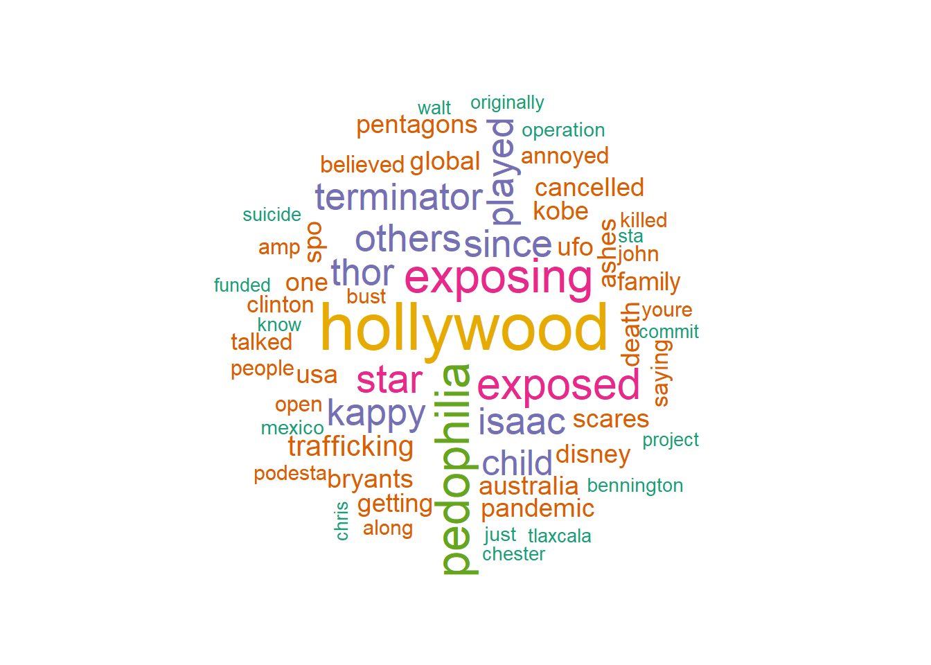
Genera diversos wordclouds y graba en disco el wordcloud generado. Busca información de paquete wordcloud2. Genera algún gráfico con este paquete.
frecuencias.df <- as.data.frame(names(freq2))
frecuencias.df <- cbind(frecuencias.df, freq2)

names(frecuencias.df) <- c("word", "freq")

head(frecuencias.df)
## word freq
## eyes eyes 42
## open open 278
## pill pill 34
## red red 42
## take take 52
## time time 64
Para las 5 palabras más importantes de vuestro análisis encontrar palabras que estén relacionadas y guárdalas en un data.frame. Haz plot de las asociaciones.
asoc <- frecuencias.df %>%
  dplyr::arrange(desc(freq))

palabras <- asoc$word[1:5]
palabras <- as.character(palabras)
palabras
## [1] "hollywood" "pedophilia" "exposing" "exposed" "star"Calculamos ahora las asociaciones con la palabra hollywood:
## $hollywood
##      isaac      kappy     others     played       star terminator       thor
##       0.99       0.99       0.99       0.99       0.99       0.99       0.99
##      since    exposed   exposing pedophilia
##       0.98       0.88       0.81       0.81
lista.asoc <- lapply(asociaciones, function(x) data.frame(rhs = names(x), cor = x, stringsAsFactors = FALSE))
lista.asoc## $hollywood
## rhs cor
## isaac isaac 0.99
## kappy kappy 0.99
## others others 0.99
## played played 0.99
## star star 0.99
## terminator terminator 0.99
## thor thor 0.99
## since since 0.98
## exposed exposed 0.88
## exposing exposing 0.81
## pedophilia pedophilia 0.81## lhs rhs cor
## 1 hollywood isaac 0.99
## 2 hollywood kappy 0.99
## 3 hollywood others 0.99
## 4 hollywood played 0.99
## 5 hollywood star 0.99
## 6 hollywood terminator 0.99
## 7 hollywood thor 0.99
## 8 hollywood since 0.98
## 9 hollywood exposed 0.88
## 10 hollywood exposing 0.81
## 11 hollywood pedophilia 0.81ggplot(df.asoc, aes(y = df.asoc[, 2])) + geom_point(aes(x = df.asoc[, 3]),
data = df.asoc[,2:3], size = 3) +
ggtitle(paste(palabras[1], "relacionado con...")) +
xlab("Correlación") +
ylab("Palabras") +
theme_gdocs()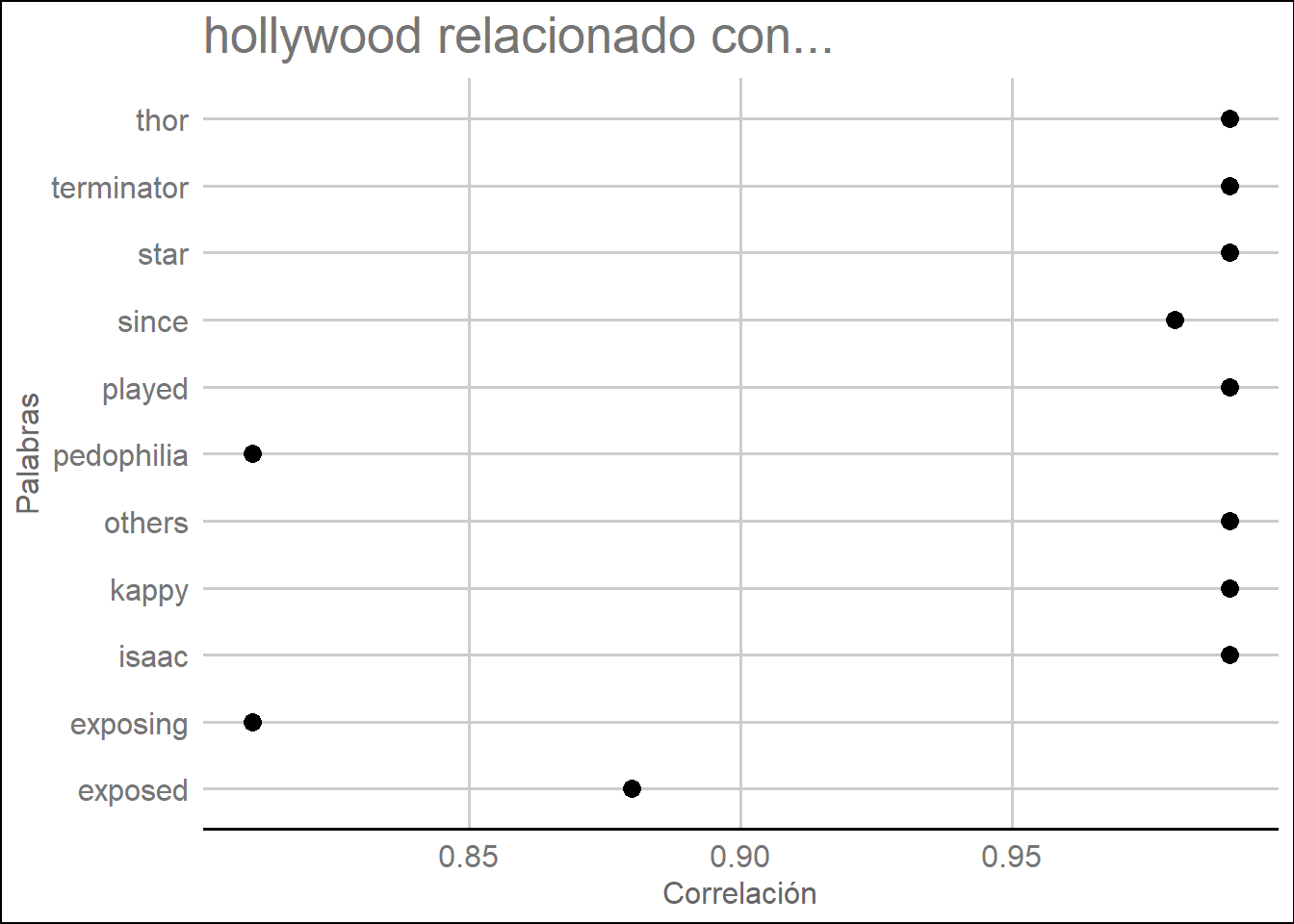
## $pedophilia
##      isaac      kappy     others     played terminator       thor  hollywood
##       0.82       0.82       0.82       0.82       0.82       0.82       0.81
##      since       star
##       0.81       0.79
lista.asoc <- lapply(asociaciones, function(x) data.frame(rhs = names(x), cor = x, stringsAsFactors = FALSE))
lista.asoc## $pedophilia
## rhs cor
## isaac isaac 0.82
## kappy kappy 0.82
## others others 0.82
## played played 0.82
## terminator terminator 0.82
## thor thor 0.82
## hollywood hollywood 0.81
## since since 0.81
## star star 0.79## lhs rhs cor
## 1 pedophilia isaac 0.82
## 2 pedophilia kappy 0.82
## 3 pedophilia others 0.82
## 4 pedophilia played 0.82
## 5 pedophilia terminator 0.82
## 6 pedophilia thor 0.82
## 7 pedophilia hollywood 0.81
## 8 pedophilia since 0.81
## 9 pedophilia star 0.79ggplot(df.asoc, aes(y = df.asoc[, 2])) + geom_point(aes(x = df.asoc[, 3]),
data = df.asoc[,2:3], size = 3) +
ggtitle(paste(palabras[2], "relacionado con...")) +
xlab("Correlación") +
ylab("Palabras") +
theme_gdocs()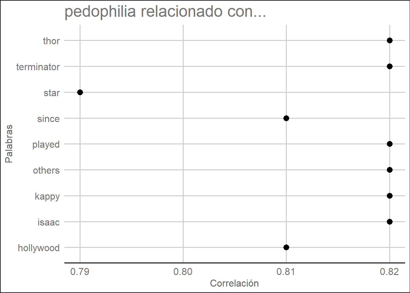
## $exposing
##      isaac      kappy     others     played terminator       thor  hollywood
##       0.82       0.82       0.82       0.82       0.82       0.82       0.81
##      since       star
##       0.81       0.79
lista.asoc <- lapply(asociaciones, function(x) data.frame(rhs = names(x), cor = x, stringsAsFactors = FALSE))
lista.asoc## $exposing
## rhs cor
## isaac isaac 0.82
## kappy kappy 0.82
## others others 0.82
## played played 0.82
## terminator terminator 0.82
## thor thor 0.82
## hollywood hollywood 0.81
## since since 0.81
## star star 0.79# Crear un dataframe con tres columnas
df.asoc <- dplyr::bind_rows(lista.asoc[1], .id = "lhs")
df.asoc## lhs rhs cor
## 1 exposing isaac 0.82
## 2 exposing kappy 0.82
## 3 exposing others 0.82
## 4 exposing played 0.82
## 5 exposing terminator 0.82
## 6 exposing thor 0.82
## 7 exposing hollywood 0.81
## 8 exposing since 0.81
## 9 exposing star 0.79ggplot(df.asoc, aes(y = df.asoc[, 2])) + geom_point(aes(x = df.asoc[, 3]),
data = df.asoc[,2:3], size = 3) +
ggtitle(paste(palabras[3], "relacionado con...")) +
xlab("Correlación") +
ylab("Palabras") +
theme_gdocs()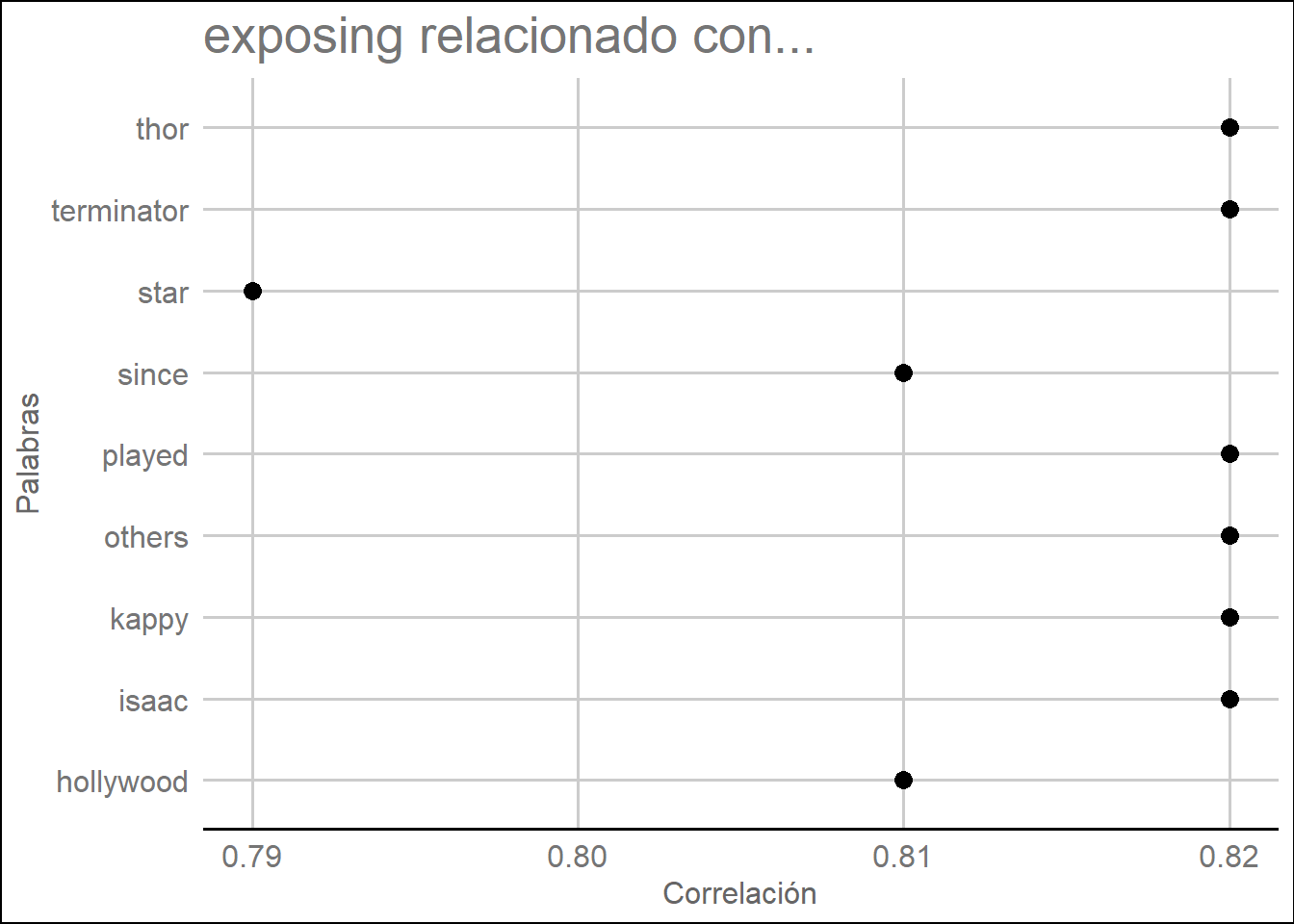
NOTA: Sólo mostramos 3 ya que todas siguen el mismo procesamiento.
Haz plot con los dispositivos desde los que se han mandado los tweets.
# plot por emisor
# encode tweet source as iPhone, iPad, Android or Web

encodeSource <- function(x) {
  if(x=="<a href=\"http://twitter.com/download/iphone\" rel=\"nofollow\">Twitter for iPhone</a>"){
    gsub("<a href=\"http://twitter.com/download/iphone\" rel=\"nofollow\">Twitter for iPhone</a>", "iphone", x,fixed=TRUE)
  }else if(x=="<a href=\"http://twitter.com/#!/download/ipad\" rel=\"nofollow\">Twitter for iPad</a>"){
    gsub("<a href=\"http://twitter.com/#!/download/ipad\" rel=\"nofollow\">Twitter for iPad</a>","ipad",x,fixed=TRUE)
  }else if(x=="<a href=\"http://twitter.com/download/android\" rel=\"nofollow\">Twitter for Android</a>"){
    gsub("<a href=\"http://twitter.com/download/android\" rel=\"nofollow\">Twitter for Android</a>","android",x,fixed=TRUE)
  } else if(x=="<a href=\"http://twitter.com\" rel=\"nofollow\">Twitter Web Client</a>"){
    gsub("<a href=\"http://twitter.com\" rel=\"nofollow\">Twitter Web Client</a>","Web",x,fixed=TRUE)
  } else if(x=="<a href=\"http://www.twitter.com\" rel=\"nofollow\">Twitter for Windows Phone</a>"){
    gsub("<a href=\"http://www.twitter.com\" rel=\"nofollow\">Twitter for Windows Phone</a>","windows phone",x,fixed=TRUE)
  }else if(x=="<a href=\"http://dlvr.it\" rel=\"nofollow\">dlvr.it</a>"){
    gsub("<a href=\"http://dlvr.it\" rel=\"nofollow\">dlvr.it</a>","dlvr.it",x,fixed=TRUE)
  }else if(x=="<a href=\"http://ifttt.com\" rel=\"nofollow\">IFTTT</a>"){
    gsub("<a href=\"http://ifttt.com\" rel=\"nofollow\">IFTTT</a>","ifttt",x,fixed=TRUE)
  }else if(x=="<a href=\"http://earthquaketrack.com\" rel=\"nofollow\">EarthquakeTrack.com</a>"){
    gsub("<a href=\"http://earthquaketrack.com\" rel=\"nofollow\">EarthquakeTrack.com</a>","earthquaketrack",x,fixed=TRUE)
  }else if(x=="<a href=\"http://www.didyoufeel.it/\" rel=\"nofollow\">Did You Feel It</a>"){
    gsub("<a href=\"http://www.didyoufeel.it/\" rel=\"nofollow\">Did You Feel It</a>","did_you_feel_it",x,fixed=TRUE)
  }else if(x=="<a href=\"http://www.mobeezio.com/apps/earthquake\" rel=\"nofollow\">Earthquake Mobile</a>"){
    gsub("<a href=\"http://www.mobeezio.com/apps/earthquake\" rel=\"nofollow\">Earthquake Mobile</a>","earthquake_mobile",x,fixed=TRUE)
  }else if(x=="<a href=\"http://www.facebook.com/twitter\" rel=\"nofollow\">Facebook</a>"){
    gsub("<a href=\"http://www.facebook.com/twitter\" rel=\"nofollow\">Facebook</a>","facebook",x,fixed=TRUE)
  }else {
    "others"
  }
}pizzagate$tweetSource = sapply(pizzagate$statusSource,
function(sourceSystem) encodeSource(sourceSystem))
ggplot(pizzagate[pizzagate$tweetSource != 'others',],
aes(tweetSource)) + geom_bar(fill = "aquamarine4") +
theme(legend.position="none",
axis.title.x = element_blank(),
axis.text.x = element_text(angle = 45, hjust = 1)) +
ylab("Number of tweets")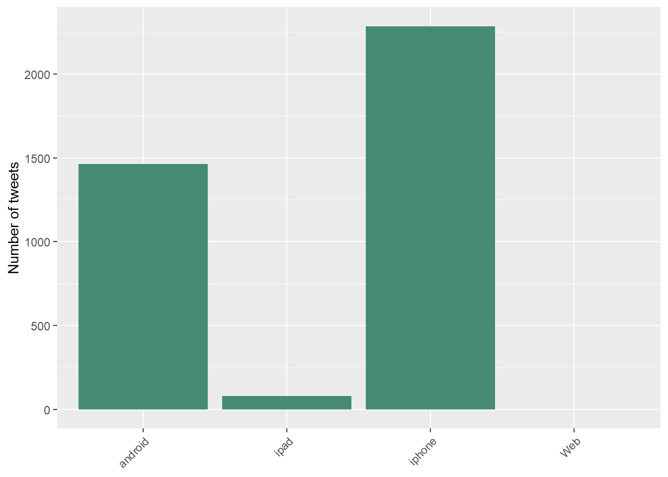
Para la palabra más frecuente de tu análisis busca y graba en un data.frame en los tweets en los que está dicho término. El data.frame tendrá como columnas: término, usuario, texto.
termino <- palabras[1]

ind <- which(grepl(termino, pizzagate$text))

hollywood <- pizzagate[ind, ]

hollywood <- hollywood %>%
  dplyr::select(screenName, text) %>%
  dplyr::mutate(termino)

knitr::kable(head(hollywood))| screenName | text | termino |
|---|---|---|
| _Phenomish | RT : Since they exposing hollywood Pedophilia. Isaac Kappy a hollywood star who played in Thor, Terminator and others exposed To | hollywood |
| Wura_zinariya | RT : Since they exposing hollywood Pedophilia. Isaac Kappy a hollywood star who played in Thor, Terminator and others exposed To | hollywood |
| YungGuille | RT : Since they exposing hollywood Pedophilia. Isaac Kappy a hollywood star who played in Thor, Terminator and others exposed To | hollywood |
| OpenUp40 | RT : Since they exposing hollywood Pedophilia. Isaac Kappy a hollywood star who played in Thor, Terminator and others exposed To | hollywood |
| ConnieAmaya4 | RT : Since they exposing hollywood Pedophilia. Isaac Kappy a hollywood star who played in Thor, Terminator and others exposed To | hollywood |
| 07V7 | RT : Since they exposing hollywood Pedophilia. Isaac Kappy a hollywood star who played in Thor, Terminator and others exposed To | hollywood |
Se repite mucho el tweet debido a ser bastante viral (el método searchTwitter permite recoger el mismo tweet al ser retweeteado muchas veces), por ello se repite mucho en nuestro dataset donde aparece la palabra Hollywood.
- Quitamos los paquetes debido a que surgen conflictos entre funciones que se llaman igual, con el objetivo de que compile el book completo.