Documento 22 Analisis con TidyText
22.1 El formato tidy
Tal y como está descrito en Hadley Wickham (Wickham 2014), tidy data tiene la siguiente estructura:
- Cada variable es una columna
- Cada observación es una fila
- Cada unidad de análisis es una tabla
- Por tanto, el formato tidy text es a table with one-token-per-row: - Un token es una unidad de texto con significado: una palabra, o varias (depende del análisis que estemos haciendo).
Tokenizar es el proceso de dividir el texto en tokens. Los tokens pueden ser por tanto:
- una palabra
- dos palabras (bi-gram)
- n palabras (n-gram)
- una frase
- un párrafo
Una vez que el texto se ha transformado a formato tidy se analizará y transformará.
Fases en análisis de texto con tidy text:
- Tokenizar: unnest_tokens
- Usar dplyr, tidyr, etc. Repetir 2 hasta conseguir formato tydy text.
- Análisis de frecuencias: contar, resumenes de textos (dplyr). Repetir 3 hasta que el texto esté limpio (preprocesamiento)
- Visualizar: ggplot
- Extraer conocimiento
22.2 Análisis
Continuando con el análisis del conjunto de tweets anterior…
Aplciar el análisis de textos que hemos visto en clase usando tidytext.
22.2.1 Tokenizar.
## Warning: Missing column names filled in: 'X1' [1]## Parsed with column specification:
## cols(
## X1 = col_double(),
## text = col_character(),
## favorited = col_logical(),
## favoriteCount = col_double(),
## replyToSN = col_character(),
## created = col_datetime(format = ""),
## truncated = col_logical(),
## replyToSID = col_double(),
## id = col_double(),
## replyToUID = col_double(),
## statusSource = col_character(),
## screenName = col_character(),
## retweetCount = col_double(),
## isRetweet = col_logical(),
## retweeted = col_logical(),
## longitude = col_logical(),
## latitude = col_logical()
## )pizzagate <-
mis_tweets %>%
mutate(text = str_replace_all(text, '(<a href=\"|http|https|" rel=\"nofollow\">|</a>)[^([:blank:]|\\"|<|&|#\n\r)]+', ""))
#pizzagate$text <- gsub("http.*","", pizzagate$text)
#pizzagate$text <- gsub("https.*","", pizzagate$text)
#pizzagate$text <- gsub(x = pizzagate$text, pattern = "[0-9]+|[[:punct:]]|\\(.*\\)", replacement = "")
mis_tokens <- pizzagate %>%
unnest_tokens(word, text)
mis_tokens## # A tibble: 90,987 x 17
## X1 favorited favoriteCount replyToSN created truncated
## <dbl> <lgl> <dbl> <chr> <dttm> <lgl>
## 1 1 FALSE 0 <NA> 2020-06-01 08:03:19 FALSE
## 2 1 FALSE 0 <NA> 2020-06-01 08:03:19 FALSE
## 3 1 FALSE 0 <NA> 2020-06-01 08:03:19 FALSE
## 4 1 FALSE 0 <NA> 2020-06-01 08:03:19 FALSE
## 5 1 FALSE 0 <NA> 2020-06-01 08:03:19 FALSE
## 6 1 FALSE 0 <NA> 2020-06-01 08:03:19 FALSE
## 7 1 FALSE 0 <NA> 2020-06-01 08:03:19 FALSE
## 8 1 FALSE 0 <NA> 2020-06-01 08:03:19 FALSE
## 9 1 FALSE 0 <NA> 2020-06-01 08:03:19 FALSE
## 10 1 FALSE 0 <NA> 2020-06-01 08:03:19 FALSE
## # ... with 90,977 more rows, and 11 more variables: replyToSID <dbl>, id <dbl>,
## # replyToUID <dbl>, statusSource <chr>, screenName <chr>, retweetCount <dbl>,
## # isRetweet <lgl>, retweeted <lgl>, longitude <lgl>, latitude <lgl>,
## # word <chr>## [1] "X1" "favorited" "favoriteCount" "replyToSN"
## [5] "created" "truncated" "replyToSID" "id"
## [9] "replyToUID" "statusSource" "screenName" "retweetCount"
## [13] "isRetweet" "retweeted" "longitude" "latitude"
## [17] "word"#Eliminamos la lista de palabras vacías. Vemos tamaño antes y después.
data("stop_words")
rbind(head(stop_words), tail(stop_words))## # A tibble: 12 x 2
## word lexicon
## <chr> <chr>
## 1 a SMART
## 2 a's SMART
## 3 able SMART
## 4 about SMART
## 5 above SMART
## 6 according SMART
## 7 you onix
## 8 young onix
## 9 younger onix
## 10 youngest onix
## 11 your onix
## 12 yours onix## [1] 90987mis_tokens <- mis_tokens %>%
anti_join(tibble(word = tm::stopwords("es")))%>%
anti_join(tibble(word = tm::stopwords("en")))%>%
anti_join(tibble(word = tm::stopwords("french")))## Joining, by = "word"
## Joining, by = "word"
## Joining, by = "word"## [1] 60740Inspeccionamos las palabras y miramos algunas que haya que limpiar
## [1] "rt"              "benjamincespe17" "take"            "red"
## [5] "pill" "time"## [1] 60740## # A tibble: 3,550 x 2
## word n
## <chr> <int>
## 1 rt 4297
## 2 pizzagate 2429
## 3 hollywood 1354
## 4 __blalock 955
## 5 pedophilia 903
## 6 anonymous 902
## 7 exposing 898
## 8 exposed 786
## 9 star 683
## 10 since 660
## # ... with 3,540 more rows- Evolución Miramos fecha en la que se bajaron los tweets para hacer una evolución temporal:
## [1] "POSIXct" "POSIXt"## [1] "2020-05-31 20:44:57 UTC"## [1] "2020-06-01 08:03:19 UTC"Instante temporal de segundos, minutos y horas:
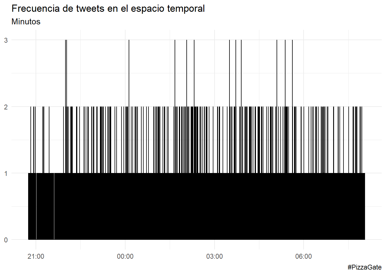
Por segundos.
## [1] 5000 17pizzagate %>%
ts_plot("seconds") +
ggplot2::theme_minimal() +
ggplot2::labs(
x = NULL, y = NULL,
title = "Frecuencia de tweets en el espacio temporal",
subtitle = "Minutos",
caption = "#PizzaGate"
)
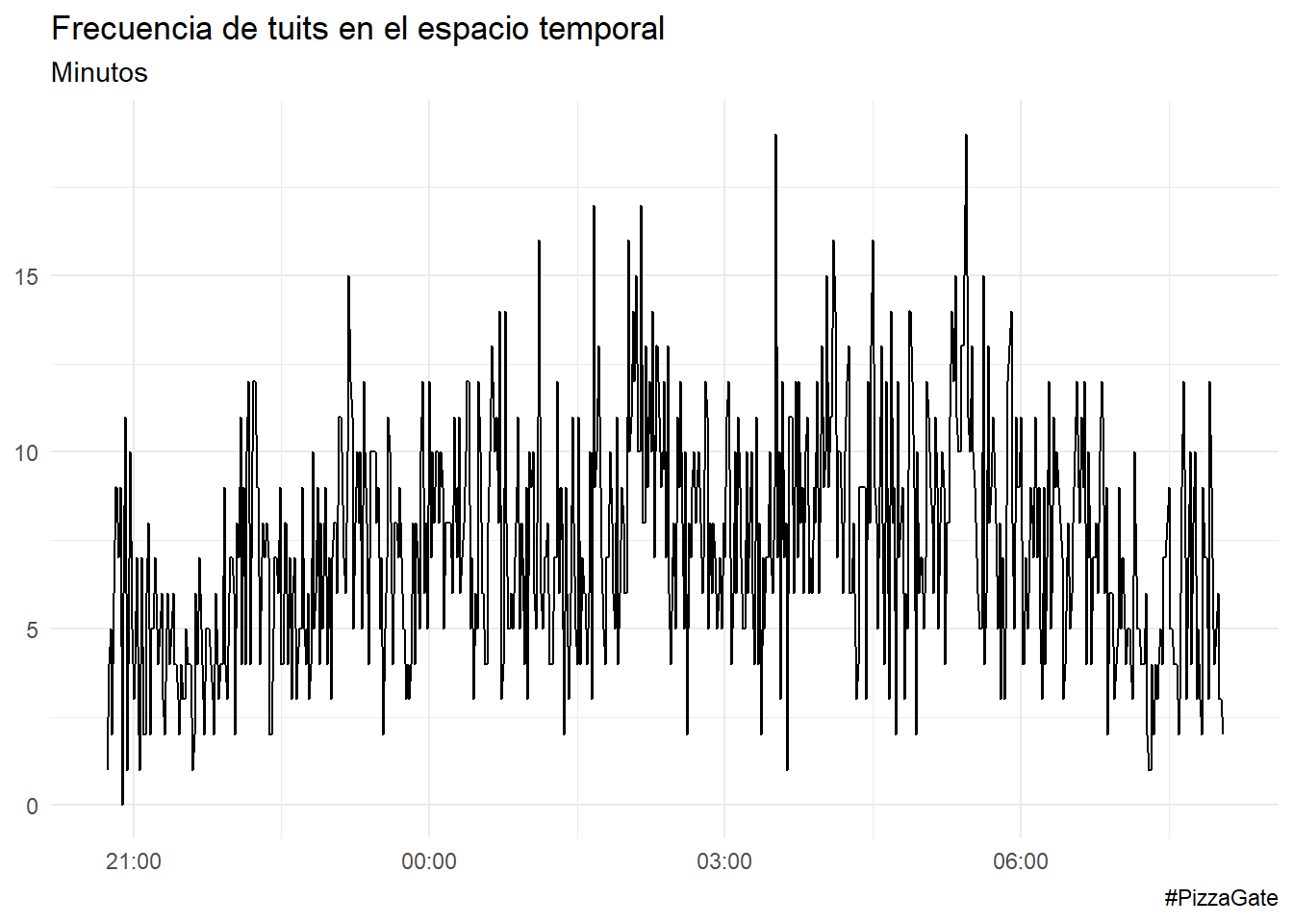
Por minutos.
pizzagate %>%
  ts_plot("minuts") +
  ggplot2::theme_minimal() +
  ggplot2::labs(
    x = NULL, y = NULL,
    title = "Frecuencia de tuits en el espacio temporal",
    subtitle = "Minutos",
    caption = "#PizzaGate"
  )
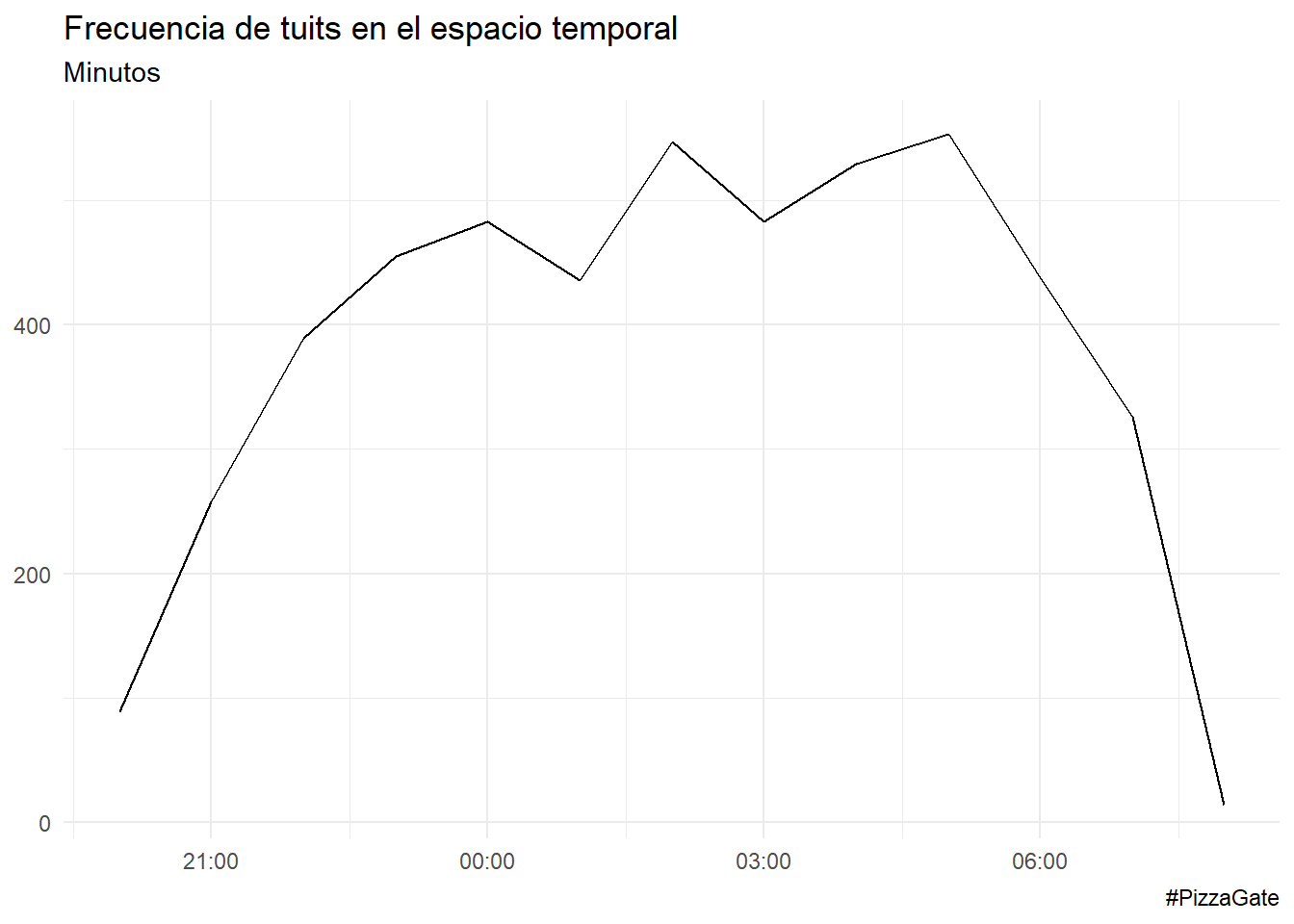
Por horas.
pizzagate %>%
  ts_plot("hours") +
  ggplot2::theme_minimal() +
  ggplot2::labs(
    x = NULL, y = NULL,
    title = "Frecuencia de tuits en el espacio temporal",
    subtitle = "Minutos",
    caption = "#PizzaGate"
  )
22.2.2 Preprocesamiento
Filtramos tokens que no tengan números (quitamos los números), eliminamos palabras individuales, me quedo con palabras con los caracteres que me interesan, eliminar algunas palabras que se detecten que no tienen sentido, etc.
mis_tokens <- mis_tokens %>%
  filter(!str_detect(word, "[0-9]"),
         word != "on",
         word != "rt",
         word != "t",
         !str_detect(word, "[a-z]_"),
         !str_detect(word, ":"))

# inspeccionar y volver a limpiar
head(mis_tokens$word,20)
## [1] "take" "red" "pill" "time" "open"
## [6] "eyes" "anonymus" "pizzagate" "whitehouse" "cafemonera"
## [11] "anonymous" "right" "now" "ignoring" "pizzagate"
## [16] "arrest" "julian" "assange" "release" "documentary"mis_tokens <- mis_tokens %>%
filter(!str_detect(word, "[0-9]"),
word != "t.co",
word != "in",
word != "https",
word != "won’t",
word != "le",
word != "los ",
word != "ass ",
word != "rt",
word != "https",
word != "pour",
word != "__blalock",
!str_detect(word, "[a-z]_"),
!str_detect(word, ":"))
# inspeccionar y volver a limpiar
head(mis_tokens$word,20) ## [1] "take" "red" "pill" "time" "open"
## [6] "eyes" "anonymus" "pizzagate" "whitehouse" "cafemonera"
## [11] "anonymous" "right" "now" "ignoring" "pizzagate"
## [16] "arrest" "julian" "assange" "release" "documentary"22.2.3 Palabras más frecuentes - wordcloud
Eliminamos las palabras vacías (usamos anti_join()):
## Joining, by = "word"## Joining, by = "word"
mis_tokens %>%
count(word, sort = TRUE) %>%
filter(n > 400) %>%
mutate(word = reorder(word, n)) %>%
ggplot(aes(word, n)) + geom_col(fill = "dodgerblue4") +
xlab(NULL) + coord_flip() + ggtitle("Palabras más comunes")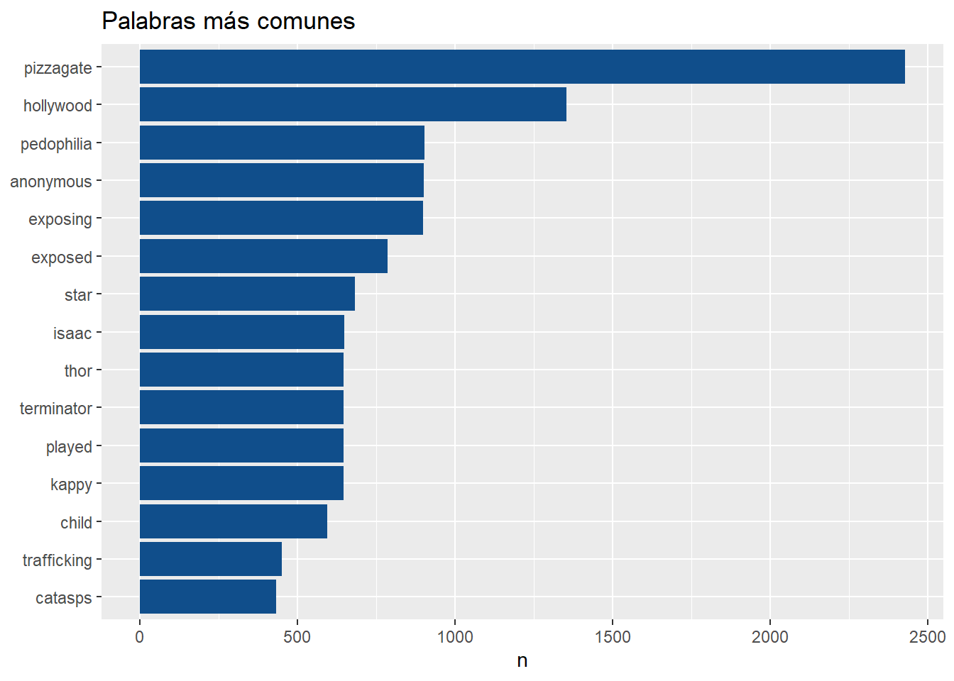
Gráficos para visualizar las palabras más frecuentes.
mis_tokens %>%
  count(word, sort = TRUE) %>%
  mutate(word = reorder(word, n)) %>%
  dplyr::filter(n > 600 ) %>%
  ggplot(aes(word, n)) +
  ggplot2::labs(
    y = "Veces que aparece",
    x = "Palabra",
    title = "Palabras más repetidas (> 400 veces)"
  ) +
  geom_col() +
  coord_flip() +
  theme_minimal()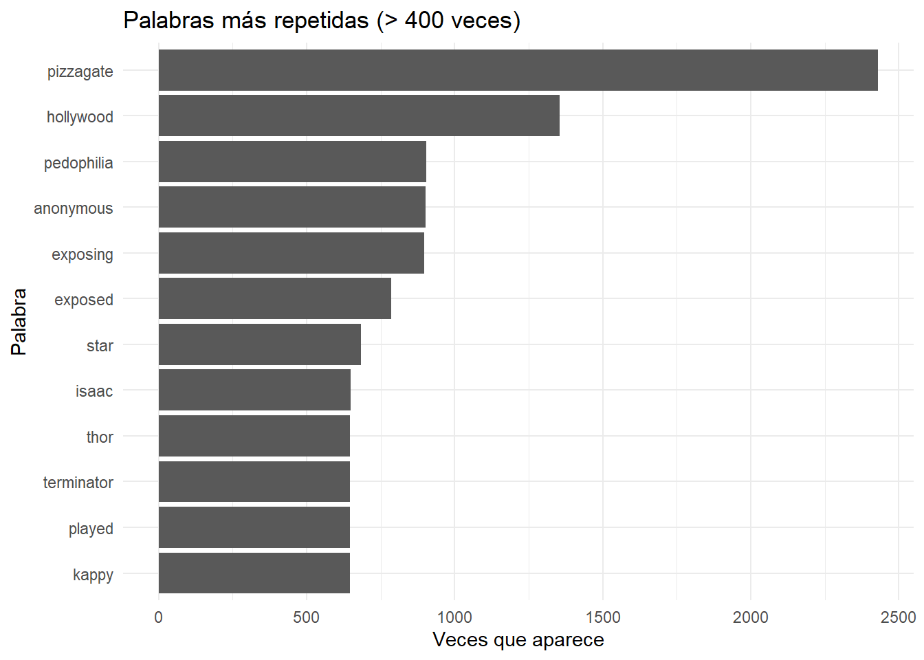
Construimos un wordcloud:
#Otras paletas:

#color_pal <- viridis::viridis(10, 1)
#color_pal <- sample(colors(),4)
#color_pal1 <- c("darkseagreen", "khaki1",       "powderblue",  "chocolate3")

color_pal1 <- c("red4","steelblue3", "red2", "grey19")

mis_tokens %>%
  count(word, sort = TRUE) %>%
  dplyr::filter(n > 50 ) %>%
  with(wordcloud::wordcloud(words = word,
                            freq = n,
                            max.words = 300,
                            random.order = FALSE,
                            rot.per = 0.25,colors = color_pal1))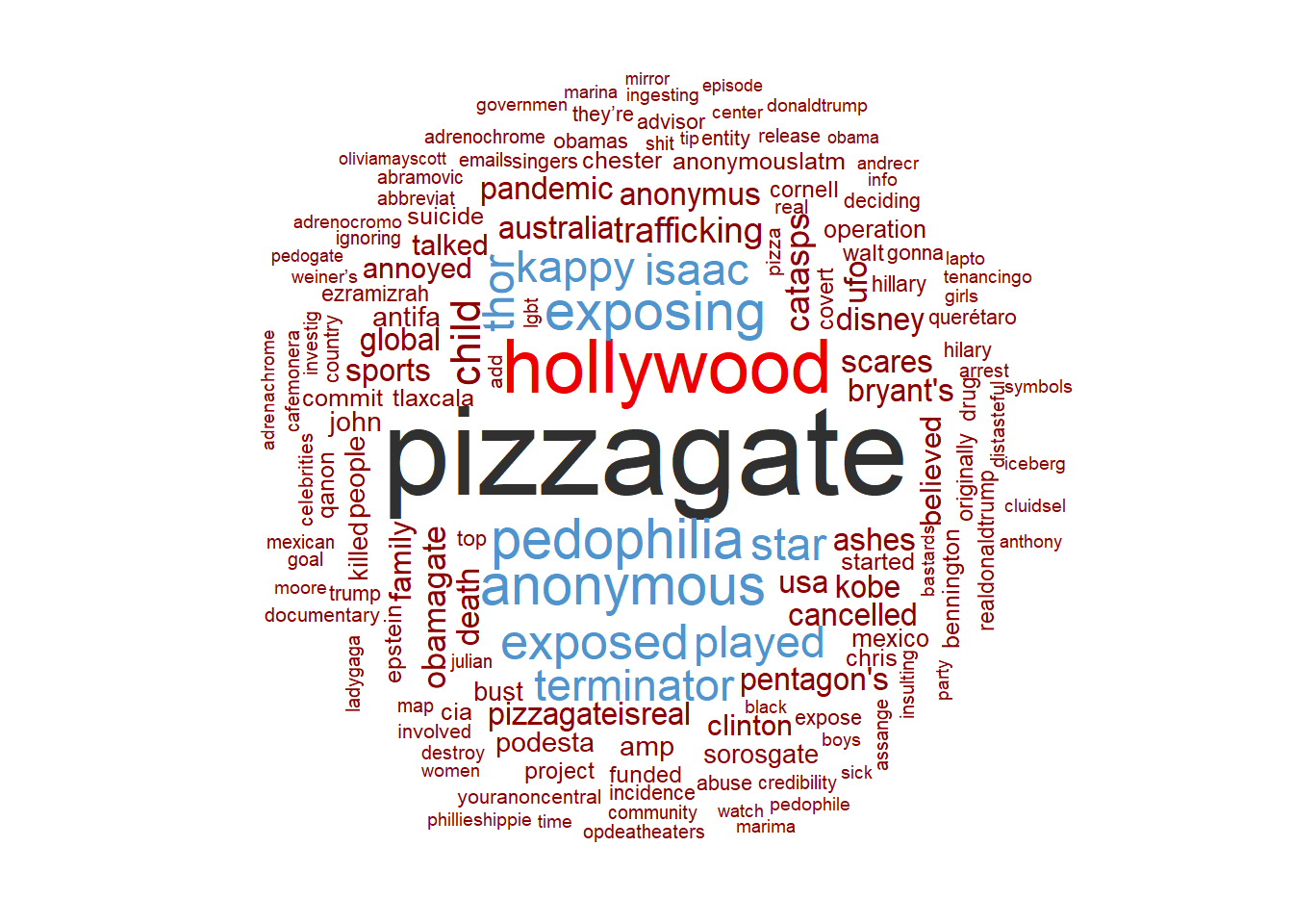
22.3 Análisis de sentimientos
Analizamos los sentimientos usando bing lexicon. Tidytext incorpora tres diccionarios de sentimientos:
- bing
- affin
- nrc
22.3.1 Bing
Bing proporciona la etiqueta de positivo o negativo a su dicionario de palabras.
La función inner_join() añade la información de sentimiento de esa palabra.
Tablas con palabras asociadas al sentimiento positivo y negativo:
## Joining, by = "word"sentiment_mis_tokens_bing %>%
summarise(Negative = sum(sentiment == "negative"),
positive = sum(sentiment == "positive"))## # A tibble: 1 x 2
## Negative positive
## <int> <int>
## 1 2913 631sentiment_mis_tokens_bing %>%
group_by(sentiment) %>%
count(word, sort = TRUE) %>%
filter(n > 5) %>%
ggplot(aes(word, n, fill = sentiment)) + geom_col(show.legend = FALSE) +
coord_flip() + facet_wrap(~sentiment, scales = "free_y") +
ggtitle("Contribución al sentimiento") + xlab(NULL) + ylab(NULL)+
theme()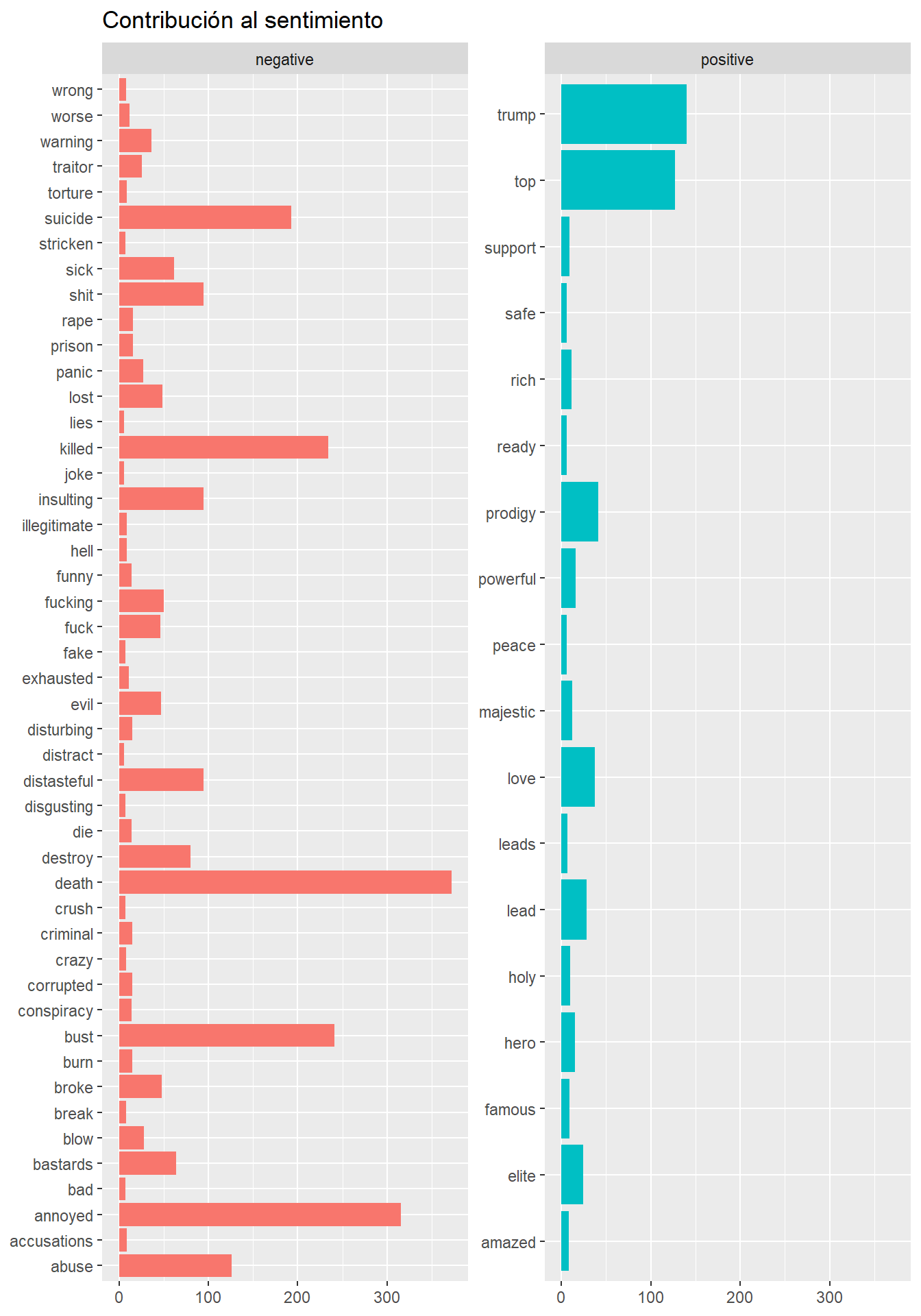
En el mismo gráfico juntamos los sentimientos positivos y negativos:
sentiment_mis_tokens_bing %>%
  group_by(sentiment) %>%
  count(word, sort = TRUE) %>%
   filter(n>25) %>%
 mutate(n = ifelse(sentiment == "negative", -n, n)) %>%

  ggplot(aes(word, n, fill = sentiment)) + geom_col() + coord_flip() +
    ggtitle("Contribución al sentimiento") +
   theme_minimal()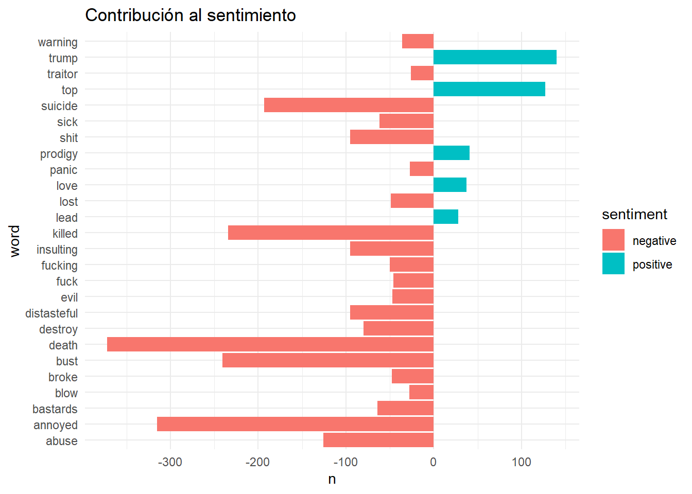
#NRC
Proporciona la etiqueta (anger, anticipation, disgust, fear, joy, negative, positive, sadness, surprise or trust) a las palabras.
Analizamos cuantas palabras aparecen con cada uno de estos sentimientos:
library(textdata)# necesario para usar nrc

sentiment_mis_tokens_nrc <-
mis_tokens %>%
  inner_join(get_sentiments("nrc")) %>%
  group_by(word, sentiment) %>%
  count(word, sort = TRUE) %>%
   filter(n > 100) %>%
  ggplot(aes(x = n, y = word, fill = n)) +
  geom_bar(stat = "identity", alpha = 0.8) +
  facet_wrap(~ sentiment, ncol = 5)
## Joining, by = "word"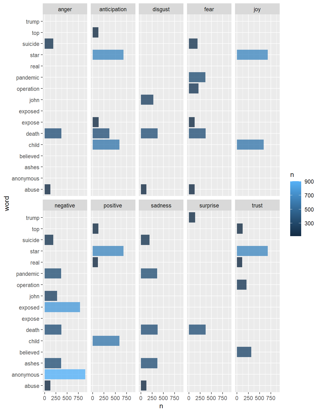
Con gráficos de barras para cada palabra:
mis_tokens %>%
  inner_join(get_sentiments("nrc")) %>%
  group_by(word, sentiment) %>%
  count(word, sort = TRUE) %>%
   filter(n > 100) %>%
  ggplot(aes(x = word, y = n)) +
  geom_bar(stat = "identity", alpha = 0.8) +
  facet_wrap(~ sentiment, ncol = 3)+
   theme(axis.text.x = element_text(angle = 90, hjust = 1))
## Joining, by = "word"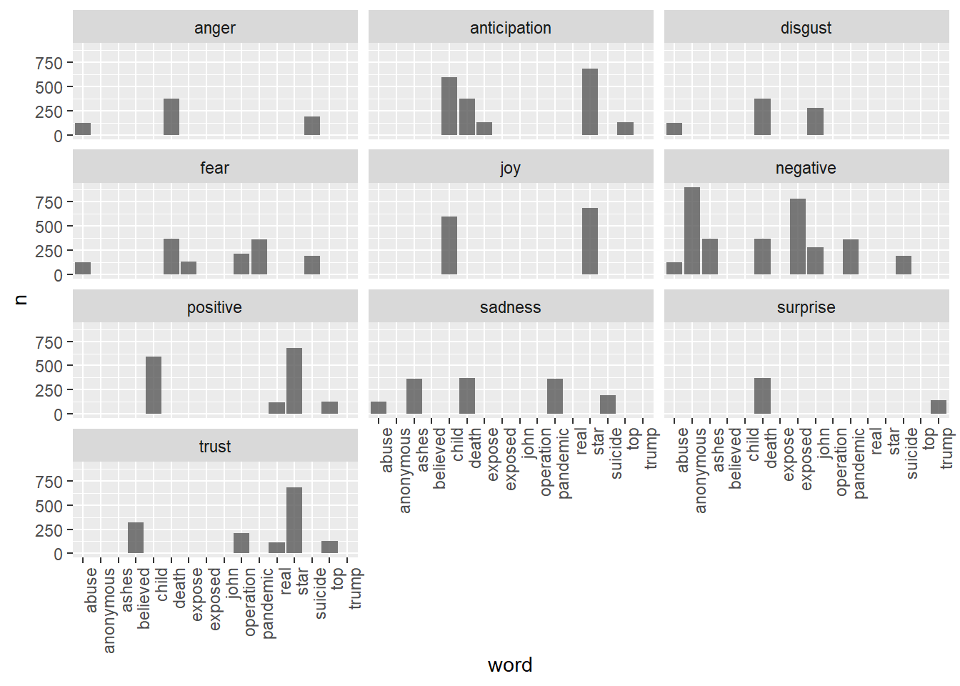
Veamos usando lexicon Afinn la evolución de los sentimientos a lo largo de los tweets:
mis_tokens_afinn <- mis_tokens %>%
   select(id, retweetCount, favoriteCount, created, retweetCount, isRetweet,
         word) %>%
  inner_join(get_sentiments("afinn"))
## Joining, by = "word"mis_tokens_afinn %>%
group_by(id, created) %>%
summarize(sentiment = mean(value)) %>%
ggplot(aes(x = created, y = sentiment)) +
geom_smooth() +
labs(x = "Date", y = "Media usando Afinn")## `geom_smooth()` using method = 'gam' and formula 'y ~ s(x, bs = "cs")'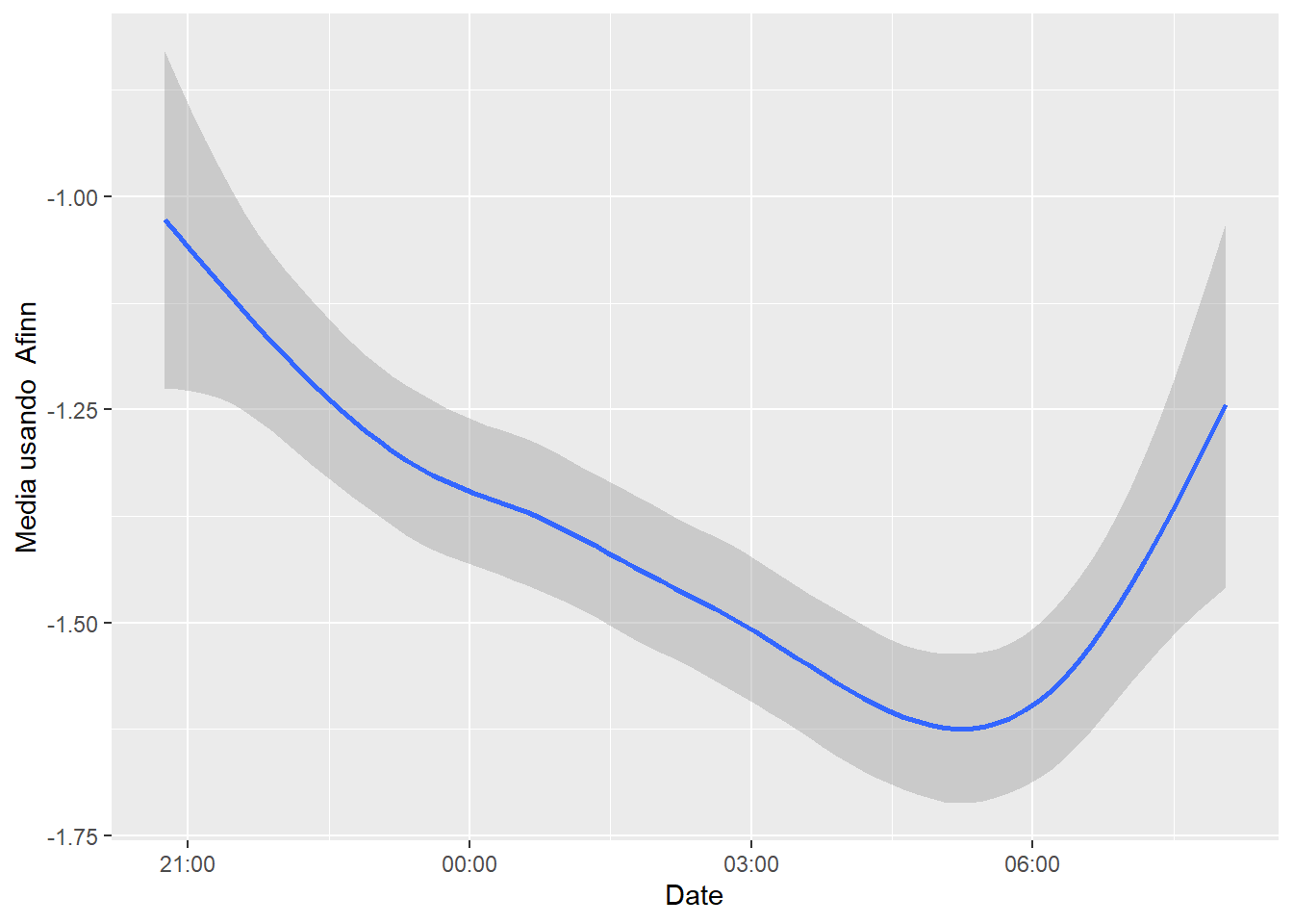
- Quitamos los paquetes debido a que surgen conflictos entre funciones que se llaman igual, con el objetivo de que compile el book completo.