Documento 15 Examen Reglas y fcaR (2)

library(arules)
library(arulesViz)
library(fcaR)

label.att <- function(n) paste0('att',n)
label.obj <- function(n) paste0('obj',n)


rbv <- function(n) sample(0:1,n,replace = T)



context.no.sparness <- function(num.obj,num.attr) {
  mi.df <- data.frame(rbv(num.obj))
  for (k in 1:(num.attr-1)){
      col <- rbv(num.obj)
      mi.df <- cbind(mi.df,col)
  }
  return(mi.df)
}#End context.no.sparness


#
#' @title Generating a random context
#' @description Algorithm for generate a random context
#' @param num.obj Number of objects for the context
#' @param num.attr Number of attributes for the context
#' @param sparness Probability that an object has an attribute
#' @param namefile Name for the output file
#' @return A data.frame with the random context and a output file
#' @export context
#' @examples
#' c <- context(3, 4, 0.2, "randomContext")
#'

context <- function(num.obj, num.attr, sparness=NULL, namefile="context") {
  if (num.obj < 1 || num.attr < 1){
    stop("The number of objects and the number of attributes must be greater than zero.")
  } 
  if (!is.null(sparness) && ((sparness < 0) || (sparness > 1))){
    stop("Sparness must be a number between 0 and 1.") 
  }
  if(is.null(sparness)){
    mi.df <- context.no.sparness(num.obj, num.attr)
  }else{
    totalN <- num.obj*num.attr
    ones <- totalN*sparness
    if(ones < totalN/2){
      mi.df <- putOnes(mi.df, totalN, ones, num.obj, num.attr)
    }else{
      mi.df <- putZeros(mi.df, totalN, (totalN-ones), num.obj, num.attr)
    }
  }
  colnames(mi.df) <- as.vector(sapply(1:num.attr,label.att))
  rownames(mi.df) <- as.vector(sapply(1:num.obj,label.obj))

  namefile <- paste(namefile, ".csv", sep="")
  write.csv(mi.df, file=namefile)
  
  return(mi.df)
}#End context



putOnes <- function(mi.df, totalN, ones, num.obj, num.attr){
  bin <- rep(0, totalN)
  contI <- 1
  contF <- num.obj
  mi.df <- data.frame(bin[contI:contF])
  for (k in seq(num.attr-1)){  
    contI <- contI+num.obj
    contF <- contF+num.obj
    col <- bin[contI:contF]
    mi.df <- cbind(mi.df,col)
  }
  numRow <- 0
  numCol <- 0
  sum <- 0
  while(sum < ones){
    numRow <- sample(1:num.obj,1)
    numCol <- sample(1:num.attr,1)
    if(mi.df[numRow,numCol] == 0){
      mi.df[numRow,numCol] <- 1
      sum <- sum + 1
    }
  }
  return (mi.df)
}#End putOnes



putZeros <- function(mi.df, totalN, zeros, num.obj, num.attr){
  bin <- rep(1, totalN)
  contI <- 1
  contF <- num.obj
  mi.df <- data.frame(bin[contI:contF])
  for (k in seq(num.attr-1)){  
    contI <- contI+num.obj
    contF <- contF+num.obj
    col <- bin[contI:contF]
    mi.df <- cbind(mi.df,col)
  }
  numRow <- 0
  numCol <- 0
  sum <- 0
  while(sum < zeros){
    numRow <- sample(1:num.obj,1)
    numCol <- sample(1:num.attr,1)
    if(mi.df[numRow,numCol] == 1){
      mi.df[numRow,numCol] <- 0
      sum <- sum + 1
    }
  }
  return (mi.df)
}#End putZeros

15.1 Dataset Mushroom

Extrae las reglas de asociación con soporte 0.28748 y confianza 0.40467 mínimas. Guardalas en una variable que se llame mis_reglas. Introduce el número de reglas obtenidas. En el Rmd, hacer un resumen de las reglas obtenidas. Explicar dicho resumen.

mush <- data(Mushroom)

mis_reglas <- apriori(Mushroom, parameter = list(supp=0.28748,conf=0.40467, minlen=2))

## Apriori
## 
## Parameter specification:
##  confidence minval smax arem  aval originalSupport maxtime support minlen
##     0.40467    0.1    1 none FALSE            TRUE       5 0.28748      2
##  maxlen target   ext
##      10  rules FALSE
## 
## Algorithmic control:
##  filter tree heap memopt load sort verbose
##     0.1 TRUE TRUE  FALSE TRUE    2    TRUE
## 
## Absolute minimum support count: 2335 
## 
## set item appearances ...[0 item(s)] done [0.00s].
## set transactions ...[114 item(s), 8124 transaction(s)] done [0.02s].
## sorting and recoding items ... [28 item(s)] done [0.00s].
## creating transaction tree ... done [0.00s].
## checking subsets of size 1 2 3 4 5 6 7 8 9 10

## Warning in apriori(Mushroom, parameter = list(supp = 0.28748, conf = 0.40467, :
## Mining stopped (maxlen reached). Only patterns up to a length of 10 returned!

##  done [0.01s].
## writing ... [14397 rule(s)] done [0.00s].
## creating S4 object  ... done [0.01s].

length(mis_reglas)

## [1] 14397

summary(mis_reglas)

## set of 14397 rules
## 
## rule length distribution (lhs + rhs):sizes
##    2    3    4    5    6    7    8    9   10 
##  311 1365 2929 3769 3238 1911  720  144   10 
## 
##    Min. 1st Qu.  Median    Mean 3rd Qu.    Max. 
##   2.000   4.000   5.000   5.226   6.000  10.000 
## 
## summary of quality measures:
##     support         confidence          lift            count     
##  Min.   :0.2875   Min.   :0.4070   Min.   :0.7557   Min.   :2336  
##  1st Qu.:0.3033   1st Qu.:0.8586   1st Qu.:1.0112   1st Qu.:2464  
##  Median :0.3240   Median :0.9441   Median :1.0849   Median :2632  
##  Mean   :0.3447   Mean   :0.8980   Mean   :1.2805   Mean   :2801  
##  3rd Qu.:0.3644   3rd Qu.:1.0000   3rd Qu.:1.4962   3rd Qu.:2960  
##  Max.   :0.9754   Max.   :1.0000   Max.   :2.9265   Max.   :7924  
## 
## mining info:
##      data ntransactions support confidence
##  Mushroom          8124 0.28748    0.40467

¿Qué lift tiene la regla número 2?. Introduce en el cuestionario el valor obtenido.

quality(mis_reglas[2])$lift

## [1] 1.021805

Ordena las reglas por lift. Muestra la cola (pero solo las últimas 4 reglas) con un solo comando (a poder ser). Muestra por pantalla los atributos de la parte izquierda de la última regla que te salga por pantalla de estas 4.

# Ordeno las relgas por lift
rules.ord <- sort(mis_reglas, by="lift")

# Muestro las últimas 4
inspect(tail(rules.ord, 4))

##     lhs                    rhs            support confidence      lift count
## [1] {GillAttached=free,                                                     
##      GillSize=broad}    => {Bruises=no} 0.2936977  0.4416883 0.7557446  2386
## [2] {GillAttached=free,                                                     
##      GillSize=broad,                                                        
##      VeilColor=white}   => {Bruises=no} 0.2936977  0.4416883 0.7557446  2386
## [3] {GillAttached=free,                                                     
##      GillSize=broad,                                                        
##      VeilType=partial}  => {Bruises=no} 0.2936977  0.4416883 0.7557446  2386
## [4] {GillAttached=free,                                                     
##      GillSize=broad,                                                        
##      VeilType=partial,                                                      
##      VeilColor=white}   => {Bruises=no} 0.2936977  0.4416883 0.7557446  2386

# Muestro la última
inspect(rules.ord[length(rules.ord)])

##     lhs                    rhs            support confidence      lift count
## [1] {GillAttached=free,                                                     
##      GillSize=broad,                                                        
##      VeilType=partial,                                                      
##      VeilColor=white}   => {Bruises=no} 0.2936977  0.4416883 0.7557446  2386

# Muestro el antecedente de la última regla
inspect(lhs(rules.ord[length(rules.ord)]))

##     items              
## [1] {GillAttached=free,
##      GillSize=broad,   
##      VeilType=partial, 
##      VeilColor=white}

Filtra las reglas obtenidas al principio con valor de estimador lift mayor que 0.7557446; las guardas en una variable rules2. Ordena estas reglas por support e introduce el valor del estimador support de la primera regla (la más importante teniendo en cuenta este estimador). En el Rmd visualiza estas reglas que se te piden en cada apartado.

rules2 <- subset(mis_reglas, subset = (lift > 0.7557446))

rules2 <- sort(rules2, by="support")

quality(rules2[1])$support

## [1] 0.9753816

Para el conjunto inicial de reglas generadas usando apriori, extrae usando los métodos del paquete arules, aquellas reglas que en la parte izquierda tenga el atributo GillAttached=free y soporte mayor que 0.3643525. Introduce cuantas reglas te han salido. En el Rmd se tienen que ver las reglas que se van pidiendo en cada apartado.

r3 <- subset(mis_reglas, subset = lhs %in% c("GillAttached=free") & support>0.3643525)
r3

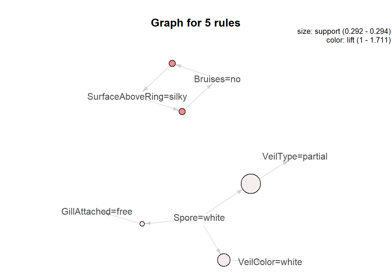
## set of 1528 rules

length(r3)

## [1] 1528

Visualizar con métodos arulesViz en forma de grafo las 5 primeras reglas obtenidas en el ejercicio. Introduce el comando en el cuestionario. Explica qué hace el comando.

Es un método de representación el cual representa las reglas como un grafo, nos muestras además las relaciones que existen entre dichas reglas.

plot(mis_reglas[1:5], method = "graph")

Ordenas las reglas extraidas inicialmente por support, selecciona el atributo que está en la derecha de la regla número 1877. Calcula en cuantas transacciones del dataset original está este atributo. Introduce este valor en el cuestionario.

rules3 <- sort(mis_reglas, by = "support")
inspect(rhs(rules3[1877]))

##     items           
## [1] {RingNumber=one}

15.2 Dataset aleatorio

Tomando como contexto formal (FC) que acabas de generar, realiza los siguientes apartados:

• Usar método de fcaR para calcular todos los conceptos. Introduce en el cuestionario cuantos conceptos has obtenido. Haz plot del contexto formal. Y dibuja el retículo de conceptos.

FC <- context(48, 20) 

fc <- FormalContext$new(FC)

# Calculamos todos las implicaciones
fc$find_concepts()

#Calculamos cúantos conceptos hemos obtenido
fc$concepts$size()

## [1] 2594

#Plot del contexto formal
fc$plot()

# Dibujamos el retículo de conceptos.
# Al ser tantos conceptos decidimos plotear los 10 primeros:
# fc$concepts$plot()

• Muestra el concepto número 3687 por pantalla. Introduce en el cuestionario el soporte de dicho concepto.

fc$concepts[3687]
fc$concepts$support()[3687]

## [1] NA

• Calcula el intent de los objetos obj22, obj36. Introduce el resultado en el cuestionario.

# Define a set of objects
S <- SparseSet$new(attributes = fc$objects)
S$assign(obj22 = 1, obj36 = 1)
S

## {obj22, obj36}

# Compute the intent of S
fc$intent(S)

## {att6, att10, att17, att18}

• Calcula las implicaciones del contexto. ¿Cuantas implicaciones se han extraido?. Introduce en el cuestionario el resultado. Muestra las 10 primeras por pantalla.

fc$find_implications()
fc$implications$cardinality()

## [1] 909

fc$implications[1:10]

## Implication set with 10 implications.
## Rule 1: {att17, att19, att20} -> {att3}
## Rule 2: {att17, att18, att19} -> {att3, att14, att15}
## Rule 3: {att16, att18, att19, att20} -> {att1, att2, att8, att11,
##   att12}
## Rule 4: {att16, att17, att18, att20} -> {att1, att2, att4, att7, att9,
##   att13}
## Rule 5: {att15, att19, att20} -> {att3, att14}
## Rule 6: {att15, att17, att20} -> {att14}
## Rule 7: {att15, att17, att19} -> {att14}
## Rule 8: {att15, att16, att20} -> {att6, att9, att18}
## Rule 9: {att15, att16, att19} -> {att14, att17}
## Rule 10: {att14, att18, att19} -> {att3, att15}

• Haz una copia (clona) el conjunto original y le das el nombre fc_2. Usando fc_2, aplica solo la regla de composición ¿Cuantas implicaciones han aparecido tras aplicar la regla?. Introduce en el cuestionario el resultado.

fc_2 <- fc$clone()

fc_2$implications$apply_rules(rules = "composition",
                            parallelize = FALSE)

## Processing batch

## --> composition: from 909 to 909 in 0.02 secs.

## Batch took 0.02 secs.

fc_2$implications$cardinality()

## [1] 909

• Extrae de todas las implicaciones la que tengan en el lado derecha de la implicación el atributo att16. Introduce el número de implicaciones que cumplen esta condición. El programa debe calcularlo. No mirar en todas las implicaciones.

# Extraer del lado derecho
rh <- fc_2$implications$filter(rhs = "att16")
rh$cardinality()

## [1] 25

• Obtén los atributos que aparezcan en todos las implicaciones. Introduce el número de estos atributos.

fc$implications$get_attributes()

##  [1] "att1"  "att2"  "att3"  "att4"  "att5"  "att6"  "att7"  "att8"  "att9" 
## [10] "att10" "att11" "att12" "att13" "att14" "att15" "att16" "att17" "att18"
## [19] "att19" "att20"