D Probability Distributions
We work with data all the time, but often we don’t think about where it comes from. To understand statistical modeling we need to understand the data generating process - we need to make assumptions about where our data came from and how it was generated. These assumptions allow us to model and answer questions and make predictions.
D.1 Random Variables
The core of the data generating process are random variables. Random variables are variables that take on different values with different probabilities. Random variables are what generates the data we work with. Random variables can be discrete or continuous, and the distribution of a random variable describes the values the random variable can take on with the associated probabilities. A simple example of a discrete random variable is given in the table below, where we specify the different values the random variable \(X\) takes on, along with the associated probabilities.
| X | Prob |
|---|---|
| -10 | 0.2 |
| 0 | 0.7 |
| 10 | 0.1 |
In general we don’t have tables like the above to work with, and we rely on recognizing that many real world phenomena can be modeled by standard, known distributions. There are many common distributions used by practitioners with names such as Bernoulli, triangular, Poisson, Cauchy, exponential, and so on. In the rest of this appendix we will look at two of the more popular common distributions, the normal and the binomial.
D.2 The Normal Distribution
Sheryl Bryan is the general manager of the NewStar Hotel. Recently many negative reviews of the hotel have appeared online, which mainly complained about the lengthy check-in process. To investigate the issue, Sheryl decides to have the bellhops collect data on total check-in times over the next month. She knows that the industry standard in her market is to have total check-in take less than fifteen minutes. The negative online reviewers typically complained that they were forced to wait for over thirty minutes, so Sheryl is curious what the data show regarding extended wait times.
The figure below is a histogram for the distribution of 300 check-ins that the bellhops collected at the NewStar Hotel.
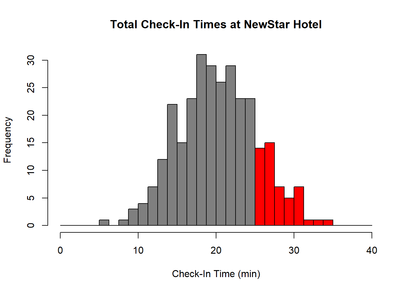
The horizontal axis shows how many minutes each customer waited to be checked-in. The left vertical axis shows the number of customers for each bin. We colored in the histogram in red for the data related to check-in times that took longer than the industry standard of twenty-five minutes.
In general, when we start talking about the chances of some event happening, we switch from a frequency histogram to a relative frequency histogram. The relative frequency of any data value is its frequency divided by the total number of data values. All of the bins of a relative frequency histogram sum to one.

We can find the proportion of check-ins that took longer than twenty-five minutes simply by adding the relative frequencies for the bins to the right of twenty-five; you can measure the graph to confirm that these bins have a total relative frequency of about 0.17, which means that about 17% of check-ins took longer than twenty-five minutes. Based on these data, a given customer at NewStar Hotel has about a 1 in 6 chance of waiting twenty-five minutes or more during check-in. Sheryl realizes from this data that she needs to investigate adding more front desk staff, or streamline check-in procedures to reduce check-in times.
When we perform statistical modeling, we consider the data generating process and often use observed data to understand the underlying theoretical distribution that produced that data. For continuous data, it is often the case that it follows a bell-shaped curve. This can be seen for the check-in data if we overlay the histogram with a smooth curve.
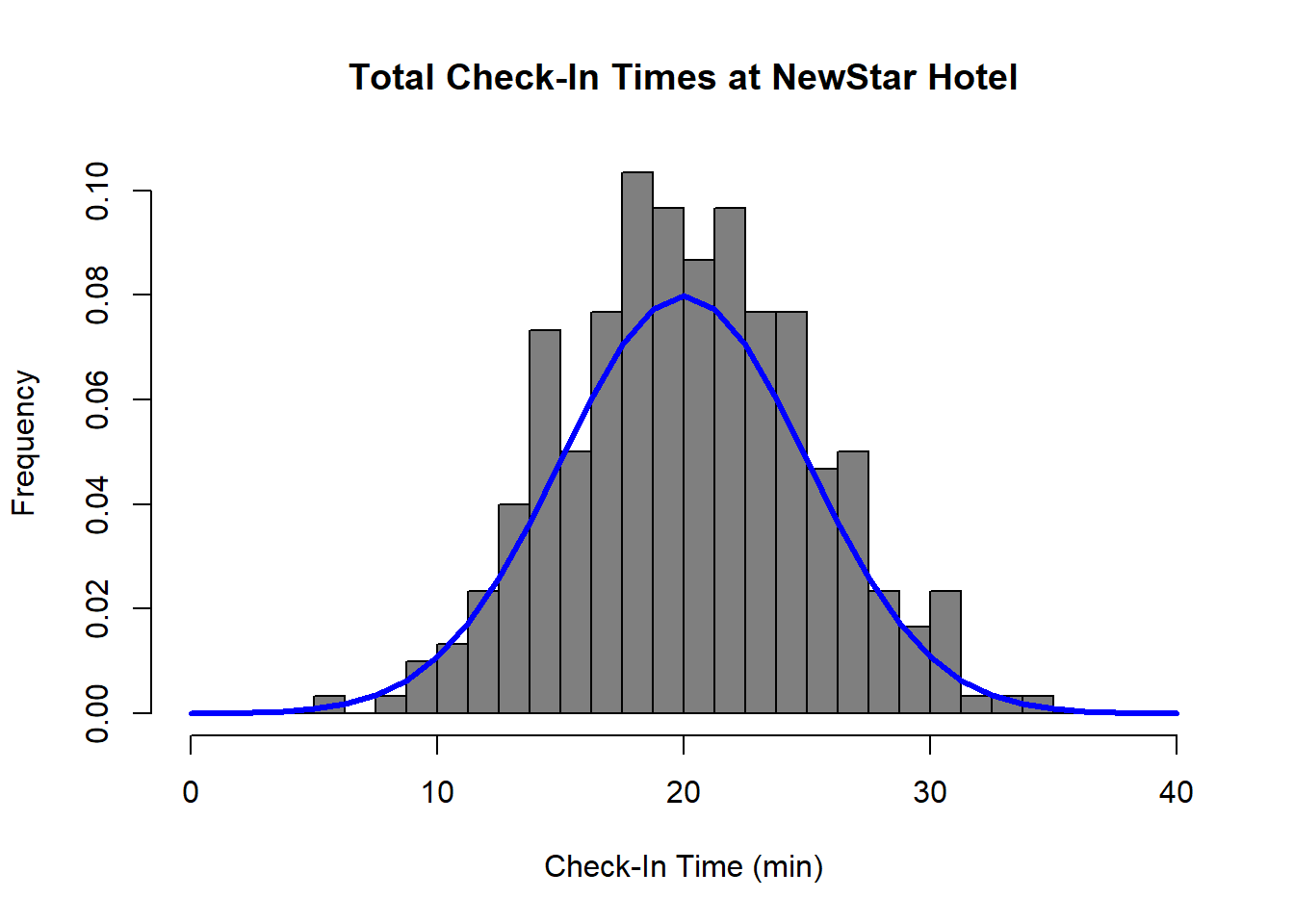
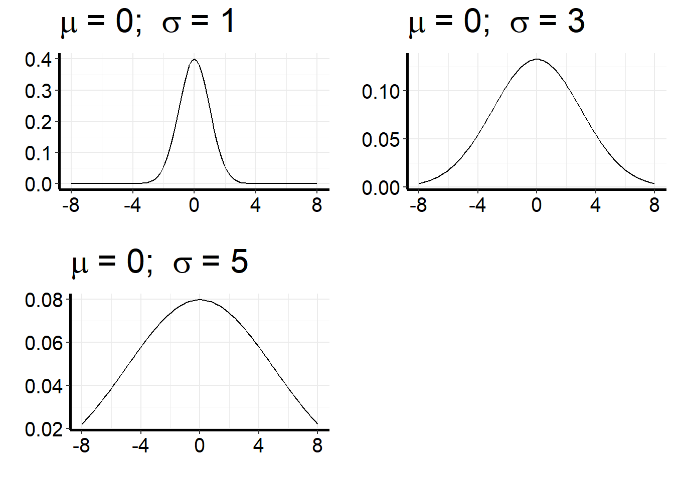
The smooth curve overlayed in the figure above is called the normal distribution. Normal distributions are characterized by their center (the mean of the distribution, denoted \(\mu\)) and their spread (denoted by the standard deviation of the distribution, \(\sigma\)). All normal distributions have the same characteristic bell shape, but they can differ in their mean and in their spread. Functions pertaining to the normal distribution are built into R. The figure below shows three different normal distributions. All have the same mean, but different variation.
D.2.1 Properties of a Normal Distribution
One useful item about the normal distribution is that if we believe our data follows a normal distribution and know the mean and standard deviation, we can understand where most of the data should lie. Under a normal distribution:
- Roughly 68% of the observed values fall within one standard deviation of the mean.
- Roughly 95% of the observed values fall within two standard deviations of the mean.
- Roughly 99.7% of the observed values fall within three standard deviations of the mean.
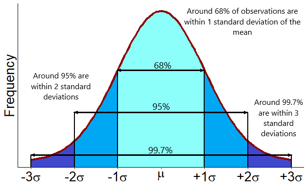
Figure D.1: The 68-95-99.7 Rule.
From this diagram, we know that if we see observations more than three standard deviations from the mean they are unusual and would be considered outliers (assuming our data is known to be normal, of course).
D.2.2 Finding Normal Probabilities
If we believe that our data follow a normal distribution, we can find the probability that an outcome lies within a given range. Because we are talking about continuous outcomes when we deal with the normal distribution, we can never evaluate the chance that we equal any outcome exactly. We can only talk about the chance that an outcome is in a range.
In R, if we have a variable \(X\) that follows a normal distribution with mean \(\mu\) and standard deviation \(\sigma\), we can use the pnorm() function to find the probability that \(X\) is less than some value a:
pnorm(a, mean, sd)
- Required arguments
a: The value of \(X\) we are testing.mean: The mean (\(\mu\)) of the distribution.sd: The standard deviation (\(\sigma\)) of the distribution.
For example, suppose the first serve speed of Tennis pro Roger Federer is normally-distributed, with a mean (\(\mu\)) of 188 km per hour and a standard deviation (\(\sigma\)) of 7 km per hour. If we want to find the probability that Federer’s next serve is under 200 kph, we need to calculate the area under the under the normal curve below 200 (i.e., the area shaded in grey):
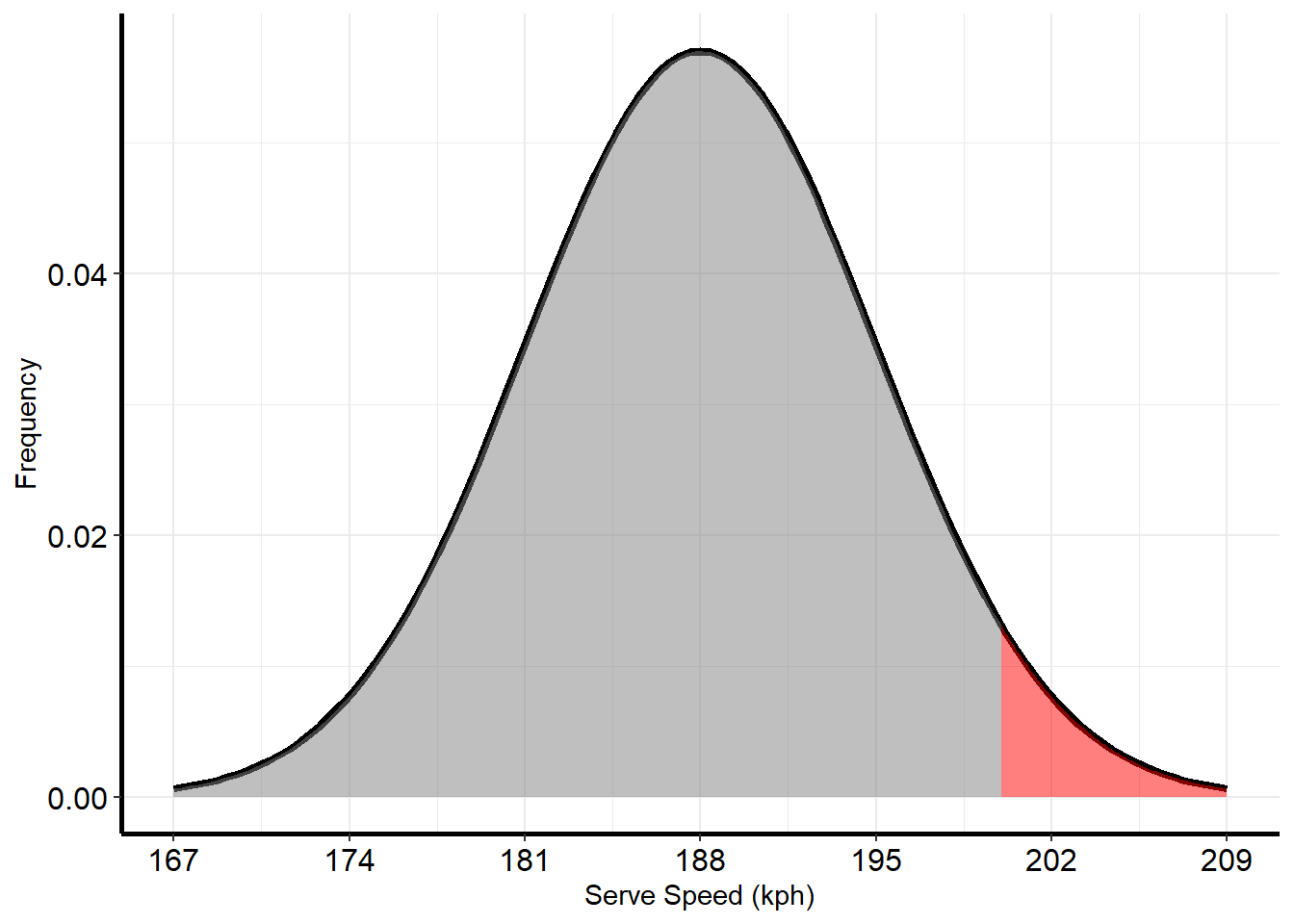
Using the pnorm() function:
pnorm(200, 188, 7)## [1] 0.9567619Conversely, to find the chance that Federer’s next serve is greater than 200 km per hour (i.e., the area shaded in red), we can simply subtract the previous probability from one:
1 - pnorm(200, 188, 7)## [1] 0.04323813Now imagine that we wanted to calculate the chance that Federer’s next serve is between 175 and 195 kph, or the area shown in blue below.
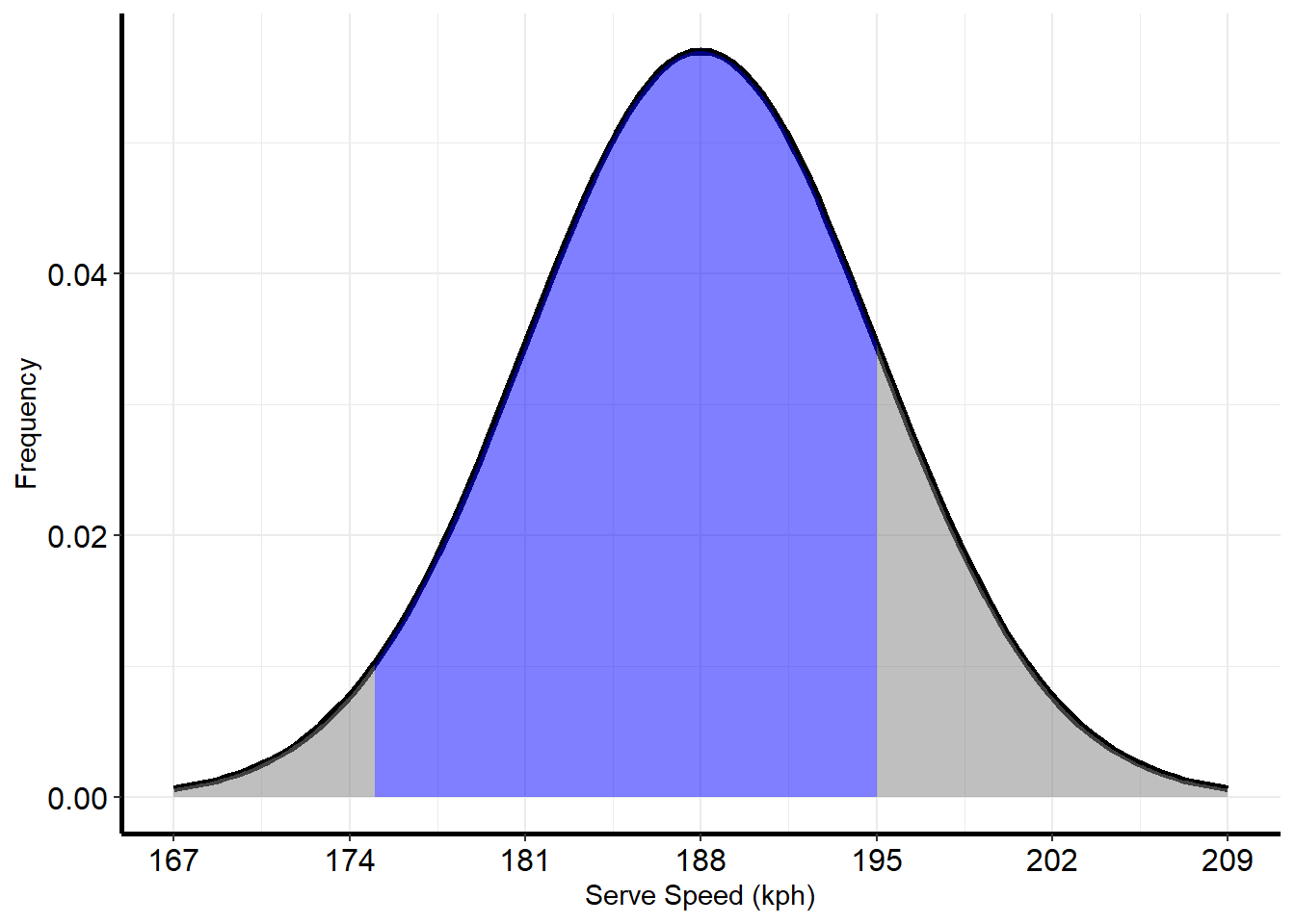
We can calculate this by finding the area below 195, and subtracting from it the area below 175:
pnorm(195, 188, 7) - pnorm(175, 188, 7)## [1] 0.8096993D.2.3 Simulating Normal Data
Sometimes we know that a process follows the normal distribution with a certain mean and standard deviation, and want to simulate data from such a distribution. A common example would be in finance when we want to simulate stock returns. The R command rnorm() will generate \(n\) random values from the specified normal distribution.
rnorm(n, mean, sd)
- Required arguments
n: The number of random values to generate.mean: The mean (\(\mu\)) of the distribution to generate data from.sd: The standard deviation (\(\sigma\)) of the distribution to generate data from.
For example, suppose we believe yearly returns of the Standard and Poor’s stock market index follows a normal distribution with mean 9% and standard deviation 23%. In the code cell below, we generate 100 years of stock market returns and plot them with a histogram. Note that since we are generating random data every time we run this R code, we will almost certainly get different values each time. The set.seed() command is used to make sure we can reproduce our random results (if we want).
set.seed(2020)
returns <- rnorm(100,9,23)
hist(returns)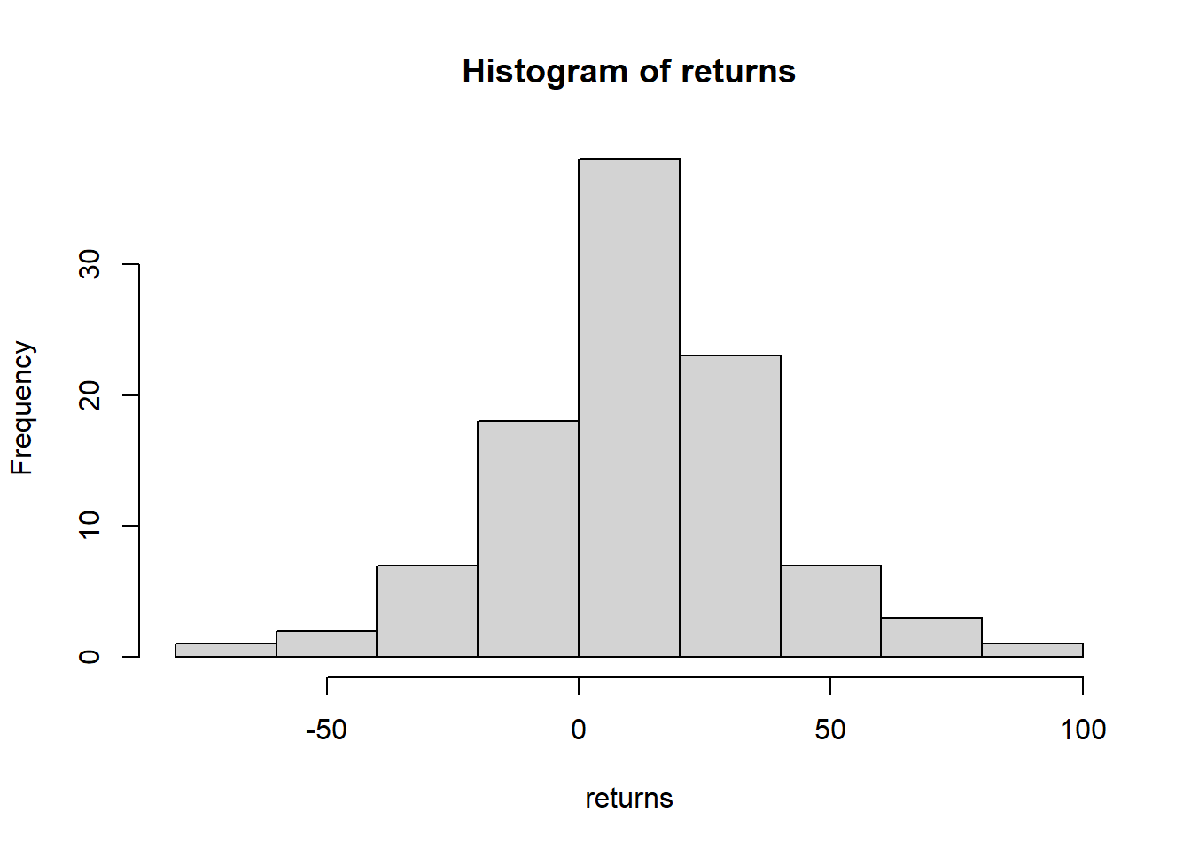
D.3 The Binomial Distribution
While the normal distribution is the most popular distribution to describe continuous random outcomes, the binomial distribution is the most popular distribution for discrete outcome data. However, it is only useful for outcomes that satisfy the binomial conditions.
Before we explicitly give the binomial conditions, let’s give a basic example of when the binomial distribution is used. Suppose that in Boston, 35% of the adult population will donate money to a charitable organization that knocks on their door. If we knock on 100 random doors in Boston, what is the chance that 60 or more of the households will give a donation?
The example above illustrates several important characteristics of the binomial distribution:
- We are modeling a situation that occurs \(n\) times, where each of these \(n\) trials are independent. In our example \(n\) equals 100, and we assume that each household’s willingness to give is not related to the preference of the other 99 households.
- The probability of a “yes” response is the same for every trial. This means we must know that all 100 households each have a 35% chance of donating.
- We are trying to answer questions about how many “yes” responses will occur over \(n\) trials. In our example, we want to calculate the probability that 60 or more households out of 100 will donate.
Although these conditions sound complicated, it is analogous to simply tossing a fair coin \(n\) times and asking if a certain number of heads appeared. Since binomial situations involve two possible outcomes (e.g., heads v. tails, will donate v. will not, etc.), we arbitrarily label one of these outcomes as a “success” and the other as a “failure.” If we let \(p\) denote the probability of a success, then:
- The probability of all successes is \(p^n\).
- The probability of no successes is \((1-p)^n\).
To find the probability of one success, or two successes, or so on, we need to turn to combinatorial theory. Instead we will simply use R, which has the binomial probability formulas built in.
D.3.1 Binomial Calculations
To calculate the probability of exactly \(x\) “successes” over \(n\) trials, we can use the dbinom() function:
dbinom(x, n, p)
- Required arguments
x: The number of “successes.”n: The number of independent trials.p: The probability of a “success.”
To calculate the probability of \(x\) “successes” or fewer over \(n\) trials, we can use the pbinom() function:
pbinom(x, n, p, lower.tail=FALSE)
- Required arguments
x: The number of “successes.”n: The number of independent trials.p: The probability of a “success.”
As above, assume there is a 35% chance that a given household is willing to donate when asked. Suppose a charity knocks on twenty randomly-selected doors in Boston.
To calculate the chance that none of the households donate:
dbinom(0, 20, 0.35)## [1] 0.0001812455To calculate the chance that at most half of the households donate:
pbinom(10, 20, 0.35)## [1] 0.9468334Finally, to calculate the chance that more than five of the households donate:
1 - pbinom(5, 20, 0.35)## [1] 0.7546043