Chapter 1 Introduction to R
Given the intended audience of this book, the first question that must be answered is: why learn programming? After all, most business analysts and managers are quite proficient at Excel, which provides enough functionality for a large fraction of the data-related tasks that managers are expected to perform. With Excel alone, one can:
- Manipulate, organize, and combine data from many different sources.
- Perform statistical analyses, such as hypothesis testing and regression modeling.
- Automate basic tasks with VBA.
- Create compelling visualizations and presentation-ready exhibits.
This is an impressive set of features, and there are many circumstances where Excel is all one needs to work with data. However, there are also increasingly many circumstances where Excel is insufficient. For example, it would be difficult to do the following with Excel alone:
- Work with very large data sets.
- Perform advanced data manipulation.
- Build predictive machine learning models.
- Easily create scalable and reproducible analyses.
This may help answer why someone would want to learn programming, but we still have not answered the really important question - why would a manager want to learn programming? Most organizations have dedicated data scientists and software engineers, and if not this work can be contracted out. So why bother teaching these skills to managers, whose time may be better spent elsewhere?
The answer to this question is the belief that organizations cannot truly develop a data-driven culture unless managers at all levels of the organization have “hands-on-keyboard” experience. The ability to manage people who have these skills is no longer enough; managers must know how to work with data themselves. Of course, the goal is never to convert managers into data scientists. Instead, the goal is to turn them into data practitioners who can ask the right questions and solve basic business problems with data. The heavy lifting will always be done by professional data scientists, but the more managers are able to go hands-on with these tools and techniques, the more organizations will be able to fully realize the value of data science capabilities.
There are many different programming languages to learn, and each has their own group of vocal supporters. This book will teach basic data science using the R programming language. Once you are comfortable with the basics of R, it will be relatively easy to pick up related languages, such as Python.
1.1 What We Talk About When We Talk About R
R is a programming language and software environment that was designed for statistical computing and graphics (R Core Team 2020). In its most basic form, R looks like the following:
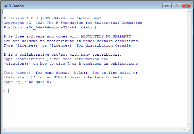
Figure 1.1: The R Console.
R commands can be entered one-by-one into the prompt (i.e., the “>”) towards the bottom left of the window.
This is the version of R you will get if you go to the official website and follow the steps to download R. However, this is not the way most people work with the R programming language. Instead, most people use one of the development environments that have been created to make it easier to write and run R code. In the same way that Microsoft Word and Apple Pages are software environments that help us write human language documents, these R development environments can help us write and run R code. Below is a brief description of the most popular development environments for R. Appendix A provides detailed instructions on how to get set up with each of these environments.
1.1.1 Jupyter Notebooks & Google Colab
Jupyter is a free, open-source application that is one of many different ways to write, run, and present R code (Jupyter Project and Community 2021). Jupyter notebooks are a particularly good option in business settings, because one can annotate code with nicely formatted images and text. This functionality can be used to create presentation-ready reports that combine code and its outputs with a written discussion of the results. Jupyter can be installed and run locally on your computer (see A.3.1).
Google Colab is a browser-based platform that allows one to create, share, edit, and run notebooks in the cloud (Colaboratory: Frequently Asked Questions 2021). In the same way that Google Docs allows one to write and share Word documents through a browser, Google Colab allows one to write, run, and share code notebooks. See A.4 for instructions on how to get started with Colab.
1.1.2 Deepnote
Deepnote is a cloud-based data analytics platform that parallels Google Colab and RStudio Cloud. The core project environment, built around Jupyter notebooks, allows users to run Python or R code. Deepnote distinguishes itself by emphasizing overall ease of use, real-time collaboration within notebooks, user-friendly file management and commenting functionality, and an active user community. It also includes more advanced features for version control, publishing, integrations with other platforms, and the like. This makes Deepnote a good option for both novice R users and educators looking for user-friendly solutions to programming, as well as advanced users working collaboratively.
1.1.3 RStudio
RStudio is another free, open-source development environment that many programmers use to develop R code (RStudio Team 2021). RStudio can be installed and run locally on your computer (see A.1.1). As shown in the figure below, the standard RStudio layout consists of four main panes:
- The Source Pane - Here you can write multiple lines of R code and then run them all at once. You can also save all the code you write in the Source pane into an R script (.R) file.
- The Console Pane - A prompt where you can enter R commands one-by-one. This may look similar to the R Console shown in Figure 1.1.
- The Environment & History Pane - In the Environment tab you can see the objects that exist within your working environment, and in the History tab you can look back through the commands you have run during the current working session.
- The Files, Plots, Etc. Pane - In the Files tab you can see your file directory, and in the Plots tab you can see any plots that you create during your working session.
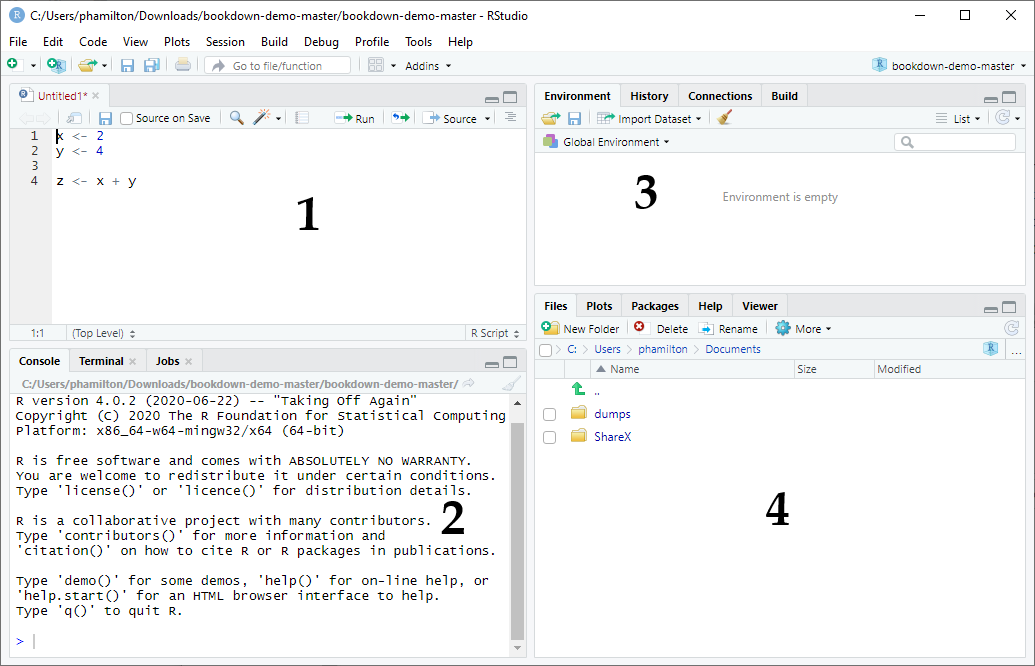
Figure 1.2: RStudio.
1.1.4 RStudio Cloud
If you do not want to run RStudio locally on your own computer, you can use RStudio Cloud (here). This service allows you to create several projects for free, but you will eventually need to pay to for your usage. See 1.1.4 for instructions on how to get started with Rstudio Cloud.
1.2 R Packages
In its most basic form, the R language contains a set of commands and functionality that are collectively referred to as base R. Any time you run R code, you will always have access to these base commands. However, you can import additional functionality by installing and loading packages, which expand what the R language can do. The R community has developed an immense number of packages that can help with nearly any type of analysis you can think of.
It is not always clear when to import a package and when to rely on base R. Your repertoire of packages will grow with experience. However, as a first step it would be helpful to review the list of the most popular R packages here. Throughout the book we will showcase a variety of different packages, many of which are on this list. Beyond the book, your best resource is Google - whenever you want to perform a new type of analysis, start by Googling to see if a relevant R package already exists.
1.2.1 Tidyverse
Throughout this book, we will rely on a collection of R packages known as the tidyverse (Wickham et al. 2019). The tidyverse packages were designed to create a streamlined workflow in R for data manipulation, exploration, and visualization. Everything that we will do with the tidyverse could be accomplished in base R. However, the tidyverse provides an elegant and efficient workflow that makes many of these tasks significantly easier and more efficient.
1.3 Reading This Book
1.3.1 Code Examples
This book contains many examples of R code, as well as the corresponding output of that code. To help distinguish between R code and regular text, all code examples are set apart in light grey boxes. For example, the following very simple code example adds two plus two:
## [1] 4The output the code produces will always be shown below the code box in a separate light grey box. In the above example, the R code 2 + 2 produces the output 4. Note that code output is typically preceded by ## [1].
1.3.2 Function Syntax
A fundamental part of R programming is the use of functions, which are very similar to functions in Excel. For example, you may be framiliar with the Excel function SUMIF(), which sums the values in a range of cells that adhere to a certain criteria. Imagine we have a data set with employee salaries at a small software company, and would like to calculate the total amount spent on employees in the Operations department:
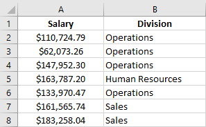
Figure 1.3: Example Excel data.
We could accomplish this in Excel with the SUMIF() function, which uses the following syntax:
SUMIF(range, criteria, sum_range)
- Required arguments
range: The range of cells where the criteria should be evaluated.criteria: The criteria to apply to the cells inrange.
- Optional arguments
sum_range: The cells to sum based on the criteria.
To apply this function to the data shown in the figure, we would write =SUMIF(B2:B8, "Operations", A2:A8), which would evaluate to $454,720.83. Feel free to verify this in Excel yourself.
Note that every time we use the SUMIF() function, we must specify the range and criteria arguments. The sum_range argument is optional, and we only need to use it if we want to sum a different set of cells than those specified in the range argument.
Whenever we introduce a new R function, we will follow the same convention shown above to demonstrate the syntax of the function. The basic syntax of the function will be shown in a light blue box marked with a book symbol, and any required and optional arguments will be described below the box.
Note that in R, optional arguments often have a default value that is used unless you specifically change that argument’s value in the function call. For example, as we’ll see later, the sort() function in R is used to sort data. If the optional descending argument of the function is set to TRUE, the data is sorted from largest to smallest, and if the descending argument is set to FALSE, the data is sorted from smallest to largest. By default, the descending argument is set to FALSE, meaning if you do not explicitly change the value of descending your data will be sorted from smallest to largest. In other words, if we just ran:
sort(data)our data would be sorted from smallest to largest. However, if we wanted to sort our data from largest to smallest, we would need to run:
sort(data, descending=TRUE)We would write the syntax for this function as follows:
sort(data, descending=FALSE, …)
- Required arguments
data: The data to be sorted.
- Optional arguments
descending: If the argument equalsTRUEthe data will be sorted from largest to smallest, and if it equalsFALSEthe data will be sorted from smallest to largest.
In the function call example, we specify the default value of the optional parameter (i.e., descending=FALSE). This is so you know what the default value of the optional parameter is. We will follow this convention throughout the book.
Above in Section 1.2 we mentioned that there are many R packages that can be imported and used to extend R’s functionality. Every time we introduce a new function that comes from an external package and is not part of base R, we will write the syntax as package::function(). For example, in Section 3.2 we will learn about the read_csv() function from the tidyverse package. We will write the syntax of this function as:
tidyverse::read_csv(file, col_names=TRUE, skip=0, …)
- Required arguments
file: The file path of the file you would like to read in. Note that the path must be surrounded in quotation marks.
- Optional arguments
col_names: When this argument isTRUE, the first row of the file is assumed to contain the column names of the data set. When it isFALSE, the first row is assumed to contain data, and column names are generated automatically (X1,X2,X3, etc.)skip: The number of rows at the top of the file to skip when reading in the data. This is useful if the first few rows of your data file have text you want to ignore.
1.3.3 Warnings
Occasionally throughout the book we will issue warnings about common pitfalls or mistakes. These warnings will be presented in light yellow boxes with a flag symbol, such as:
Example warning box.
References
Colaboratory: Frequently Asked Questions. 2021. 1600 Amphitheatre Parkway, Mountain View, California, United States: Google. https://research.google.com/colaboratory/faq.html.
Jupyter Project and Community. 2021. About Us. Project Jupyter. https://jupyter.org/about.
R Core Team. 2020. R: A Language and Environment for Statistical Computing. Vienna, Austria: R Foundation for Statistical Computing. https://www.R-project.org/.
RStudio Team. 2021. RStudio: Integrated Development Environment for R. Boston, MA: RStudio, PBC. http://www.rstudio.com/.
Wickham, Hadley, Mara Averick, Jennifer Bryan, Winston Chang, Lucy D’Agostino McGowan, Romain François, Garrett Grolemund, et al. 2019. “Welcome to the tidyverse.” Journal of Open Source Software 4 (43): 1686. https://doi.org/10.21105/joss.01686.