A Development Environments
A.1 Local RStudio
RStudio is a free, open-source software environment that you can install on your computer to write and run R code. The standard version of RStudio is a desktop application, which means that it runs locally on your machine and not in the cloud.
A.1.1 Installing RStudio
To install RStudio, complete the following steps (depending on your operating system).
A.1.1.1 Installing on PC
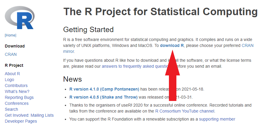
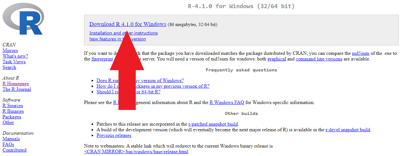
Go to the R Project’s website here: https://www.r-project.org/.
Under “Getting Started”, click “download R”.
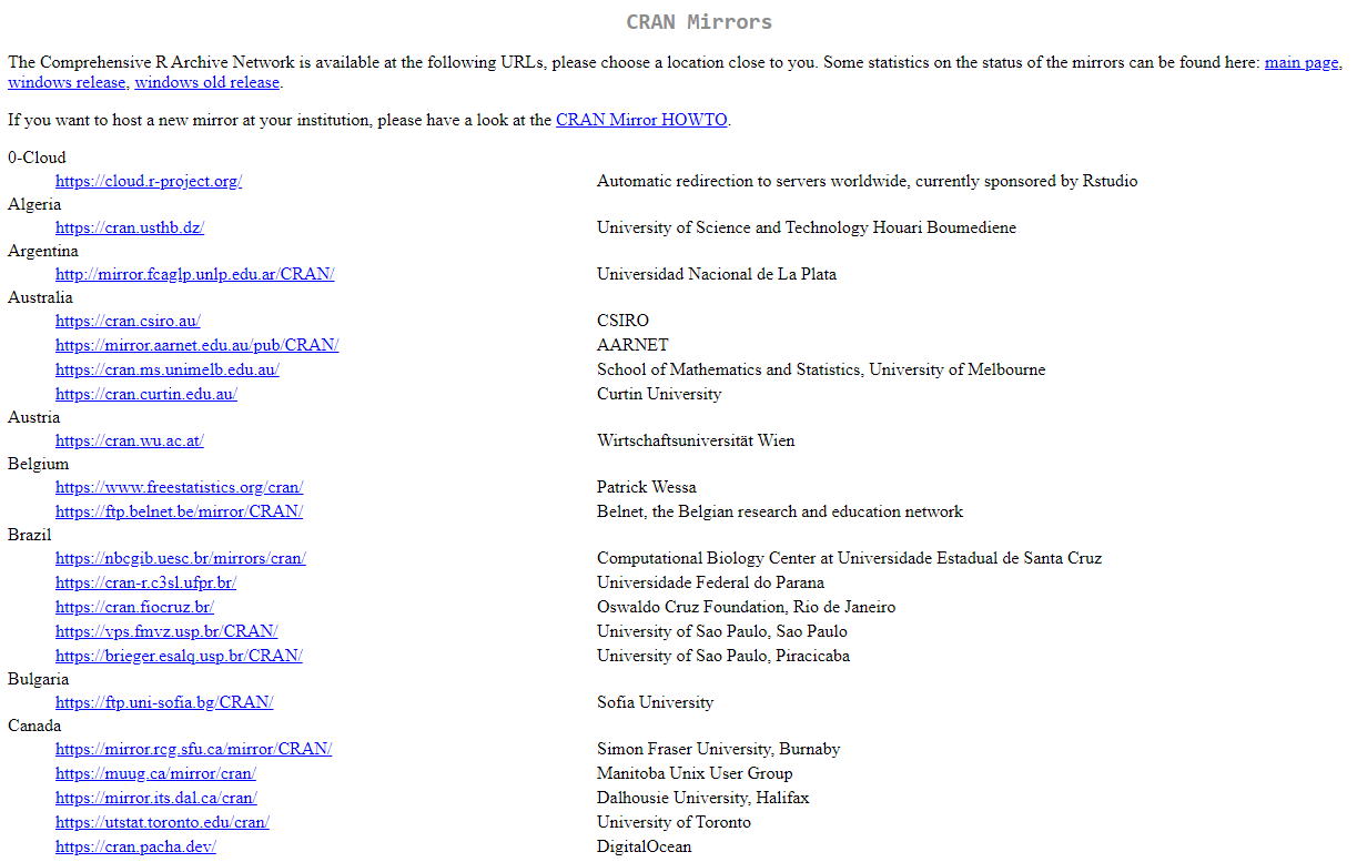
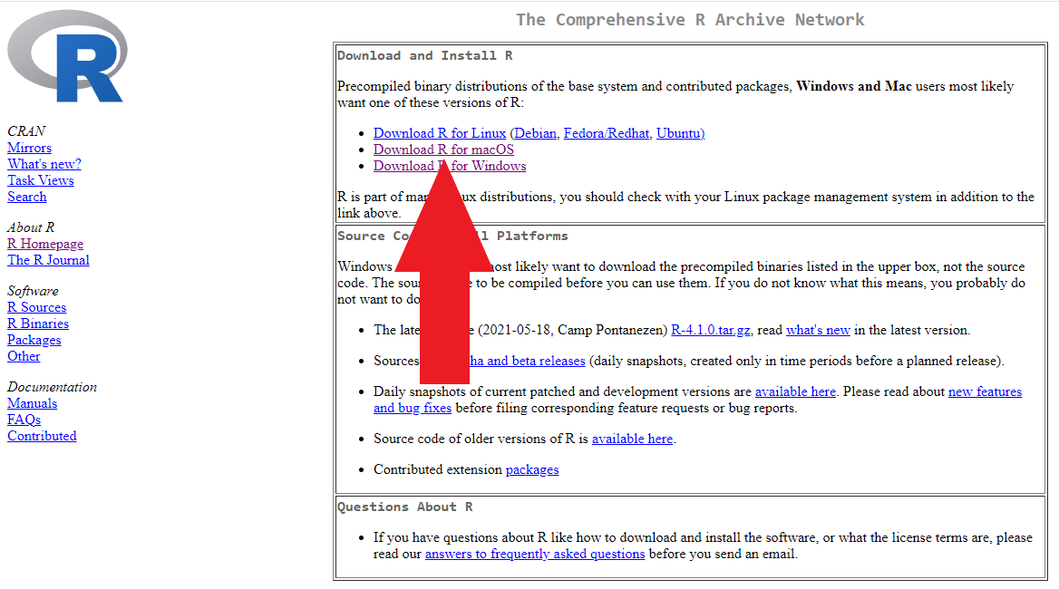
- This will direct you to a page titled “CRAN Mirrors”. On this page, find the geographic location closest to you and click the corresponding link.
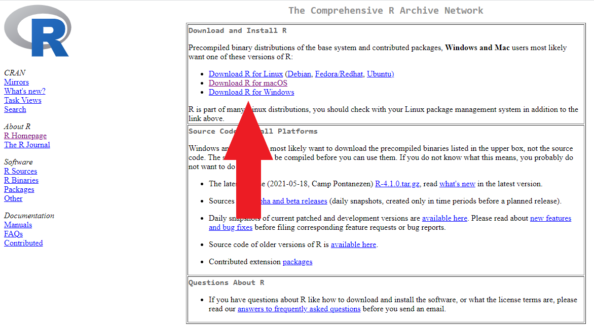
- Click “Download R for Windows” under “Download and Install R”.
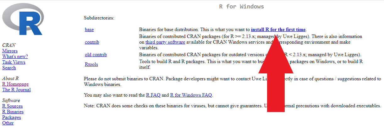
- Click “install R for the first time”.
- Click “Download R X.X.X for Windows”. Note that the version number may be different than the one shown in the screenshot below.
Run the executable (.exe) file and follow the installation instructions.
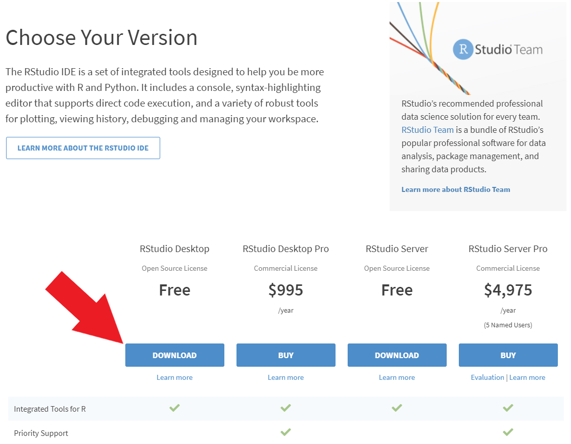
Go to the RStudio website here: http://www.rstudio.com/.
Click “DOWNLOAD”.

- Click the “DOWNLOAD” button under the free version of RStudio Desktop.
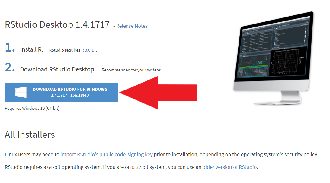
- Download the version of RStudio Desktop recommended for your system by clicking the large blue button.
- Run the executable (.exe) file and follow the installation instructions.
A.1.1.2 Installing on Mac
Go to the R Project’s website here: https://www.r-project.org/.
Under “Getting Started”, click “download R”.
- This will direct you to a page titled “CRAN Mirrors”. On this page, find the geographic location closest to you and click the corresponding link.
- Click “Download R for macOS” under “Download and Install R”.
- Click on the latest .pkg file under “Latest release”.
[ADD: screenshot]
- Open the .pkg file and follow the installation instructions.
[ADD: screenshot]
Go to the RStudio website here: http://www.rstudio.com/.
Click “DOWNLOAD”.
- Click the “DOWNLOAD” button under the free version of RStudio Desktop.
- Download the version of RStudio Desktop recommended for your system by clicking the large blue button.
[ADD: screenshot]
- Open the .dmg file and drag and drop it to the applications folder.
[ADD: screenshot]
A.1.2 Getting Started
When you launch RStudio, you should see the following basic layout:
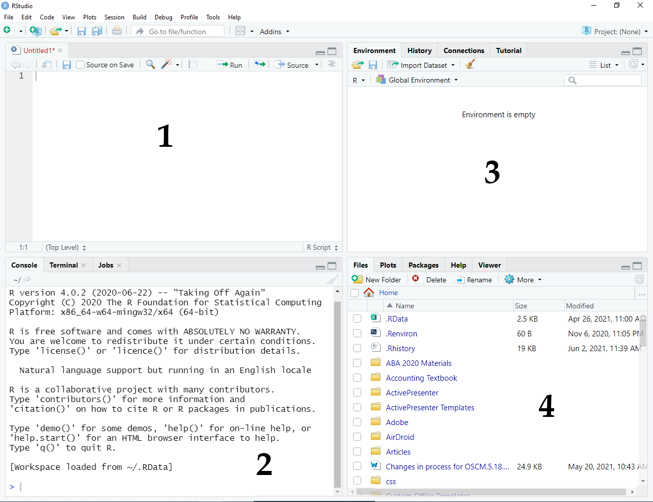
- The Source Pane
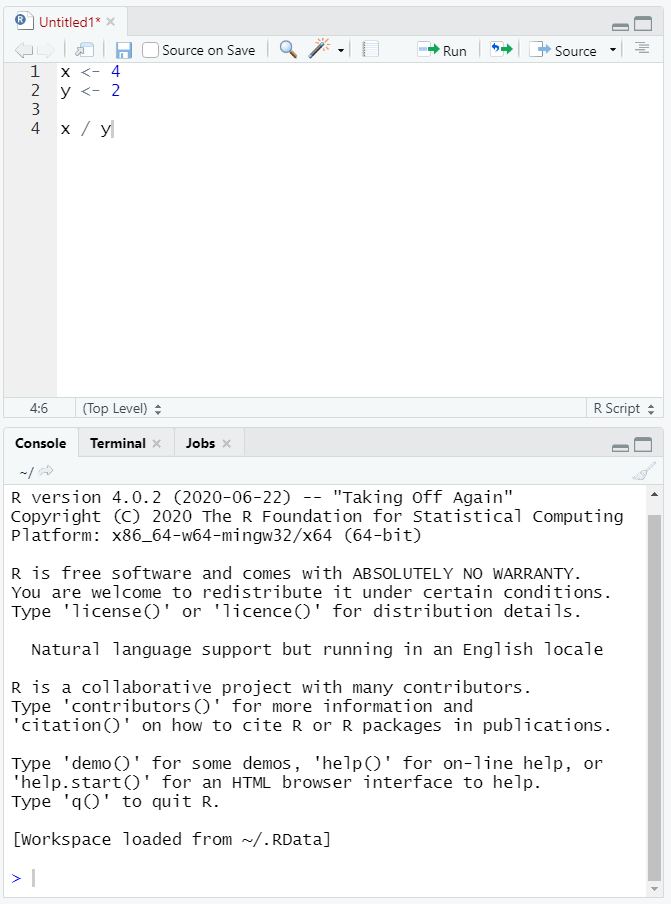
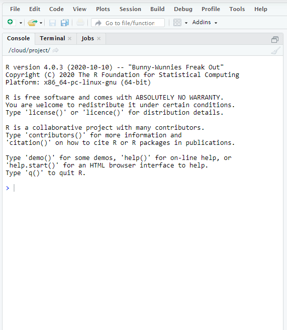
The Source pane can be used to develop R script (.R) files, which are simply text files that contain multiple lines of R code. After writing some code in the Source pane, you can highlight the lines you want to run and execute them by pressing the “Run” button. If your code produces output, it will be printed to the “Console” tab of the Console pane. For example:
To save your R script so that you can return to it later, simply click “File” -> “Save As…” in the top left of RStudio. To open an R script you had saved previously, click “File” -> “Open File…”
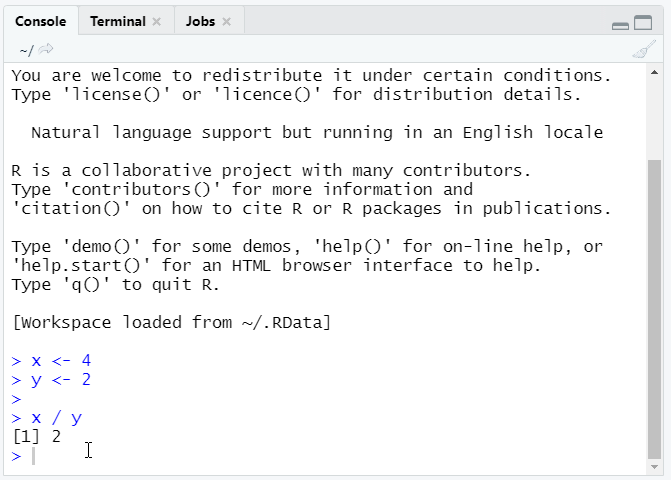
- The Console Pane
As shown above, if your code produces output it will be printed to the Console pane. Additionally, you can enter R commands one-by-one to the Console. For example:
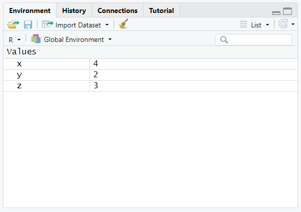
- The Environment Pane
In the Environment tab, you can see the objects that exist within your working environment. So far we have created objects called x, y, and z, so we see these in the Environment tab:
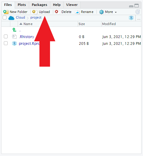
- The Files Pane
In the Files tab you can see your local file directory.
A.1.3 Reading in Data
Section 3.2 describes the different functions available in the tidyverse to read data into R. This section explains how to use those functions when working locally in RStudio.
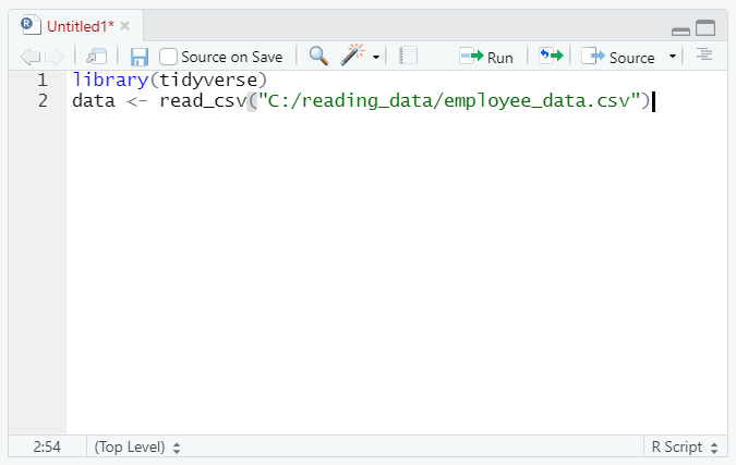
To read in data from a file, save the file on your computer and note the full file path. For example, imagine we would like to read in “employee_data.csv”, which is stored in the directory “C:/reading_data”. To read this into RStudio, we need to pass the full file path to the read_csv() function from the tidyverse package. Note that the file path needs to use forward slashes (/); you will get an error if you use backwards slashes (\).
If we don’t want to specify the full file path, we can set the folder that contains our data file as the working directory of the current session. This way, we can simply reference the file name and R will know to search for it in the folder we have set as the working directory.
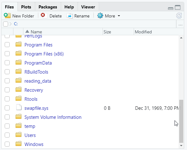
To do this, navigate to the appropriate directory in the Files pane. Then click “More” -> “Set As Working Directory”.
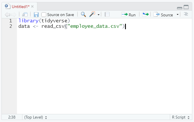
Now to read in the data you do not need to specify the full file path, you can simply pass in the name of the file:
A.2 RStudio Cloud
For a variety of reasons, you may not want to run RStudio locally on your own computer. Your machine may not have powerful enough hardware, or your computer may become sluggish if you try to get other work done while R code is running in the background. Therefore, you may instead prefer to work in the cloud. When you work in the cloud, your code is not actually running on your computer; instead, it is executed on a remote server that is managed by a cloud computing service. That way, your local computer’s resources are not occupied running your R code.
RStudio Cloud is a browser-based platform that allows you to run R code in the cloud. The interface looks nearly identical to RStudio, but you work in a web browser instead of installing RStudio locally on your computer. RStudio Cloud allows you to create several projects for free, but you will eventually need to pay to for your usage.
A.2.1 Getting Started
Start by signing up for an RStudio Cloud account here. Then read the guide to RStudio Cloud here (up to “Teaching with Cloud”).
A.2.2 Creating Projects
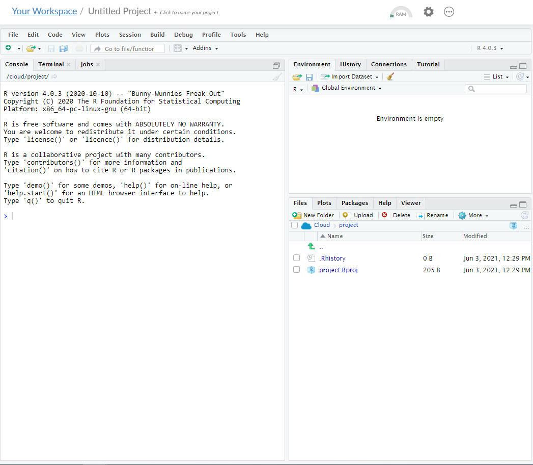
If you followed the instructions from the previous section, you should know how to create an RStudio Cloud project within your personal workspace. When you create and launch a new project, you should see the following:
To open up a new R script file within this project, click “New File” -> “R Script” directly under “File” at the top left of the screen:
The interface within an RStudio Cloud project is identical to the local interface that is explained in Section ??.
A.2.3 Reading in Data
To read data from a file, you first need to upload that file to the RStudio Cloud project. You can do this by clicking the “Upload” button at the top of the Files pane, then selecting the file from your local directory.
After you have uploaded the file to the project, you can read it into R using the functions described in Section 3.2. Note that you only need to upload files once; if you close out of the project and return to it later, any files you uploaded previously will still be accessible.
A.3 Local Jupyter Notebooks
[ADD]
A.3.1 Installing Jupyter
We will install Jupyter as part of Anaconda, a free software package that includes many different tools used by data scientists. Depending on your operating system, complete the following guides to install Anaconda on your computer:
Next, complete the following guide so that the R programming language can be used with Jupyter (by default only Python is supported).
A.3.2 Getting Started
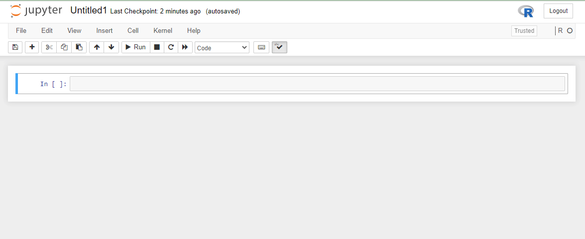
If you followed the steps in the previous section, you should now know how to launch a Jupyter notebook with the R language (Step 3 here). Launch a new notebook, and you should see the following open in your web browser:
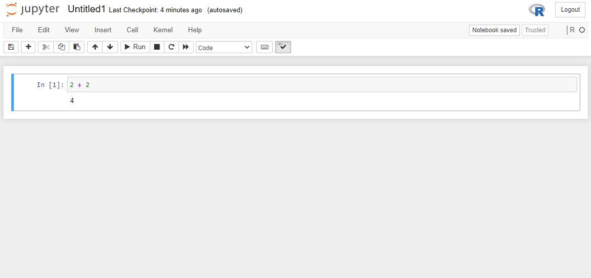
Jupyter notebooks are organized into cells. There are two primary cell types in Jupyter: code cells and markdown cells. Code cells contain R commands, which get executed when you press the “Run” button. For example, imagine we entered the R code 2 + 2 into the first code cell in our notebook. If we then press the “Run” button (or press Ctrl+Enter on the keyboard), the code will be executed and the output will be printed directly below the cell:
Markdown cells contain human language text and allow you to intersperse your R code with written commentary. For example, say that we would like to provide a written description of the operation we performed in the previous figure. To do this, we start by creating a new cell by pressing the “+” button in the top left corner of the notebook. Then, we simply change the cell type from “Code” to “Markdown” and add our written narrative to the cell. Now when we press the “Run” button, Jupyter interprets this cell as text instead of R code and formats our text nicely within the notebook.
Although it may not be obvious from this simple example, the ability to combine code and markdown cells in one document is extremely powerful. On its own, raw R code can be difficult to read and understand. Markdown allows us to complement our R code with a written narrative that provides structure to the analyses we are performing. For a more sophisticated example, see the submission to the 2019 Kaggle Machine Learning and Data Science Survey competition here.