Chapter 6 Regression Modeling
Relationships between variables are often at the heart of what we’d like to learn from data. This chapter covers regression analysis, a class of statistical methods that are used to estimate the relationship between a dependent variable and one or more independent variables. These techniques can be used to answer such questions as:
- Is there a relationship between movie box office performance and advertising spend?
- Do countries with higher GDPs have lower infant mortality rates?
- What is the relationship between a given stock’s return and the returns of the S&P 500?
- How does someone’s credit score affect the likelihood they will default on a loan?
6.1 Linear Regression
As we saw in Section 4.1.1, correlation can inform us if two variables are linearly related, and also tell us the strength and direction of the relationship. However, correlation cannot be used for any type of prediction (forecasting). Many real-world business problems are concerned with determining a relationship between a set of variables and then using that relationship for forecasting purposes. For instance, in a marketing setting, we might be interested in the relationship between the amount spent on advertising and monthly sales so that we can then do annual sales forecasting for a specified advertising budget. The method of linear regression builds upon the idea of correlation and is a modeling technique that helps us explain (predict) a dependent (or response) variable \(Y\) based on other independent (or explanatory) variables \(X\).
6.1.1 Simple Linear Regression
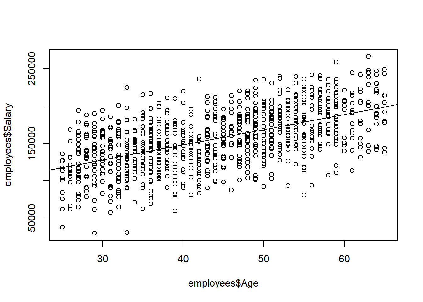
Consider the employees data and suppose we want to understand the relationship between Salary, the \(Y\) variable, and Age, the \(X\) variable. It appears to be a somewhat positive and linear relationship. The statistical technique used to fit a line to our data points is known as simple linear regression. The adjective “simple” is referring to the fact that we are using only one explanatory variable, Age, to explain at least some of the variation in the \(Y\) variable. If more than one explanatory variable is used, then the technique is known as multiple linear regression.
Formally, we assume there is a linear relationship between our variables, \(Y = \beta_0+\beta_1(X)\), but also assume there is a certain amount of “noise” (randomness) in the system that can obscure that relationship. We represent the noise by \(\epsilon\), and write:
\[Y = \beta_0+\beta_1(X)+\epsilon\]
Our goal is to find estimates of \(\beta_0\) and \(\beta_1\) using our observed data. Specifically, \(\beta_0\) is the true intercept of the linear relationship between \(X\) and \(Y\) in the population, and \(\beta_1\) is the true slope of the linear relationship between \(X\) and \(Y\) in the population. It is possible that \(\beta_1 = 0\), which would indicate there is no linear relationship between \(X\) and \(Y\). Our mission is to use the sample data to find estimates \(\beta_0\) and \(\beta_1\) and then try to determine what the true relationship is.
6.1.1.1 The Method of Least Squares
Consider the example data shown in the left plot below. On the right side plot, we have superimposed a line onto the data. For each point in the plot we can determine the vertical distance from the point to the line. We call these distances errors and denote them \(e_1,e_2,\ldots,e_6\). Note that some of these errors are positive, some are negative, and one seems to be about zero.
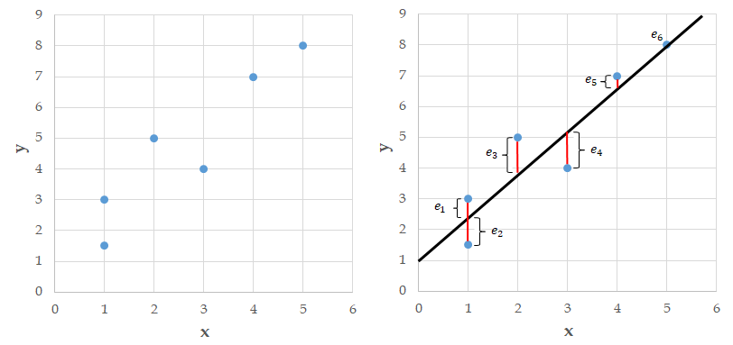
Figure 6.1: The method of least squares.
Many lines can be fit to a data set. The method of least squares finds the line that makes the sum of the squared errors as small as possible. We square the errors so negative and positive errors don’t cancel each other out. The least squares method is hundreds of years old and produces a linear fit to a data set that is both aesthetically pleasing and has nice mathematical properties.
Recall that we are assuming there is a linear relationship between our two variables, which is written as: \[Y = \beta_0+\beta_1(X)+\epsilon\]
The method of least squares gives us estimates of these population quantities so we end up with the estimated line: \[\hat{y} = b_0+b_1(x)\]
We use \(\hat{y}\) to denote an estimate of \(Y\), and \(b_0\) and \(b_1\) to denote estimates of \(\beta_0\) and \(\beta_1\), respectively.
The lm() command in R uses the method of least squares to fit a line to a given data set (the lm stands for “linear model”). This function uses the following syntax:
lm(y ~ x, data=df)
- Required arguments
y: The name of the dependent (\(Y\)) variable.x: The name of the independent (\(X\)) variable.data: The name of the data frame with theyandxvariables.
Note that when we apply lm(), we use the syntax lm(y ~ x, data=df), not lm(df$y ~ df$x). The later will work when we define the model, but will cause issues later when we try to use the model to make predictions. Therefore, never define linear regression models using the $ operator; always use the form lm(y ~ x, data=df).
Never define linear regression models with lm(df$y ~ df$x); always use the form lm(y ~ x, data=df).
Below we use lm() to fit a linear regression where \(Y\) is Salary and $X$ isAge`:
##
## Call:
## lm(formula = Salary ~ Age, data = employees)
##
## Coefficients:
## (Intercept)          Age
##       67134         2027
From this output we find that the equation of the fitted line is:
\[predicted \;salary = \hat{y} = \$67133.7 + \$2026.83(age)\]
The abline() command plots this regression line on top of our scatterplot.
abline(fit)
We say “predicted salary” because there clearly isn’t an exact relationship between Salary and Age; the regression equation just gives us a model to relate the two variables.
6.1.1.2 Interpreting Coefficients
How do we interpret the linear relationship determined by the least squares method? The slope \(b_1\) is interpreted as the average change in \(y\) for a one unit change in \(x\). Within our sample, this means that for every one-year increase in Age, on average, Salary increases by $2026.83. We also use this relationship for forecasting: we predict that, for our population, for every year increase in Age, on average, Salary will go up by $2026.83.
The intercept \(b_0\) represents the average value of \(y\) when \(x=0\). Often it is the case that we have no \(x\) values near zero, or it is not possible for \(x\) to equal zero, so the intercept is not interpretable. It is in the model to help position (or “anchor”) the line. In our example, the intercept tells us that the average Salary for someone 0 years old is $67133.7, which doesn’t make a lot of sense.
Note that although we say a change in \(x\) is associated with a change in \(y\), this does not mean that a change in \(x\) causes a change in \(y\). We can only make causal statements about our model under specific circumstances. This important distinction is discussed further in Chapter @ref{causal-inference}.
6.1.1.3 Inference for the Regression Line
Our least squares estimates \(b_0\) and \(b_1\) are estimates of the true theoretical values \(\beta_0\) and \(\beta_1\) respectively. Since the regression line is calculated using sample data, we can construct confidence intervals and perform hypothesis tests on our estimates. The confint() function reports 95% confidence intervals for the regression coefficients.
confint(fit)
##                 2.5 %    97.5 %
## (Intercept) 58390.197 75877.208
## Age          1834.364  2219.292
We can obtain more detailed output using the summary() command.
summary(fit)
##
## Call:
## lm(formula = Salary ~ Age, data = employees)
##
## Residuals:
##     Min      1Q  Median      3Q     Max
## -103272  -21766    2428   23138   90680
##
## Coefficients:
##             Estimate Std. Error t value            Pr(>|t|)
## (Intercept) 67133.70    4455.17   15.07 <0.0000000000000002 ***
## Age          2026.83      98.07   20.67 <0.0000000000000002 ***
## ---
## Signif. codes:  0 '***' 0.001 '**' 0.01 '*' 0.05 '.' 0.1 ' ' 1
##
## Residual standard error: 32630 on 918 degrees of freedom
##   (80 observations deleted due to missingness)
## Multiple R-squared:  0.3175, Adjusted R-squared:  0.3168
## F-statistic: 427.1 on 1 and 918 DF,  p-value: < 0.00000000000000022
We usually focus on just \(b_1\) since we are primarily interested in the relationship between the variables. Our best estimate for \(b_1\) is $2026.83, but because we are basing this estimate on a data sample, we could be wrong. We can say with 95% confidence that the true value of the slope (denoted \(\beta_1\)) could be as low as $1834.36 to as high as $2219.29. The good news is the confidence interval contains only positive values, indicating a positive relationship between Salary and Age. If zero fell into this interval we would not be able to conclude that there was a positive relationship between Salary and Age.
By applying the summary() command to our regression we can see p-values listed for each coefficient. The hypothesis test being done here is “does the true slope equal 0?”, and “does the true intercept equal 0?”. In symbols we are testing for the slope:
- \(H_o: \beta_1 = 0\)
- \(H_a: \beta_1 \ne 0\)
A small p-value, less than the significance level (often 0.05), means we reject the null hypothesis and can conclude there is likely a linear relationship between the \(x\) and \(y\) variables; simply put, a small p-value indicates we need \(x\) in the model.
The p-value for the intercept corresponds to the hypothesis test asking, “does the true intercept equal 0?” We often ignore the p-value of the intercept when the intercept is difficult to interpret.
6.1.1.4 The R-Squared (\(R^2\))
The summary() command gives additional information about the regression fit. In particular, at the bottom of the summary output, we see two items:
- Multiple R-squared, often denoted \(R^2\)
- Adjusted R-squared, often denoted \(R_a^{2}\)
The \(R^2\) is a goodness of fit measure and always falls in the interval 0 to 1. In essence, we do regression to try to understand how changes in the \(x\) variable explain what is happening to a \(y\) variable. If \(y\) didn’t vary when \(x\) changes, it would be very boring to explain, so in essence we are trying to explain the variation in \(y\) using \(x\). The \(R^2\) tells us the percentage of the variation in \(y\) explained by \(x\), with higher being better. One issue with \(R^2\) is that it can go up simply by adding more \(x\) variables to a model, so \(R_a^2\) reflects a penalty factor related to the number of \(x\) variables in the model. The adjusted R-squared value is always the preferred measure to report.
When a linear regression model has more than one independent variable, report \(R_a^2\) instead of \(R^2\).
However, neither \(R^2\) nor \(R_a^2\) indicates anything about predictability, so another measure described below is more useful to consider.
6.1.1.5 Estimate of Noise and Prediction
When we look at the scatter plot, we see noise in the model; that is, we see a line plus variation (“noise”) around the line. Regression modeling assumes that the noise \(\epsilon\) is normally distributed with mean 0 and variance \(\sigma^2\). The value \(\sigma^2\) is key when using a regression model for prediction, since it tells us how accurate our predictions are. The estimate of \(\sigma\) from our sample data is denoted \(s_e\) and is called the residual standard error.
This residual standard error is important because we can create approximate prediction intervals using the formula:
\[predicted\; y =\hat{y} = (b_0+b_1(x))\pm 1.96(s_e)\]
The summary() function applied to the regression tells us that the residual standard error is $32632.35. Thus, the predicted income of someone 40 years old is:
\[\$67133.7 + \$2026.83(40) = \$148206.84\]
But we know it’s not an exact relationship, so it would be nice to put lower and upper bounds on this prediction. We are roughly 95% confident that the predicted income for someone 40 years old is in the interval:
\[\$148206.84 \pm 1.96(\$32632.35) = (\$84247.43;\$212166.24)\]
A more formal prediction interval can be found in R using the predict() function. Note that the formula shown above is an approximation and that this function’s results are more precise, so the intervals differ slightly.
##        fit      lwr      upr
## 1 148206.8 84124.55 212289.1
A rough rule of thumb when looking at regression models is to look at \(s_e\) then double it; your 95% prediction interval will be roughly \(\hat{y} \pm 2(s_e)\). You can use this as a guide to decide if you think it is an acceptable model.
\(R^2\) does not inform about a linear regression model’s predictive ability, so one must also report \(s_e\).
6.1.1.6 Basic Diagnostic Plots
When doing regression analysis, we assume a linear relationship between the \(X\) and \(Y\) variable. We also assume the noise in the model follows a normal distribution. Both of these assumptions may be checked with separate diagnostic plots.
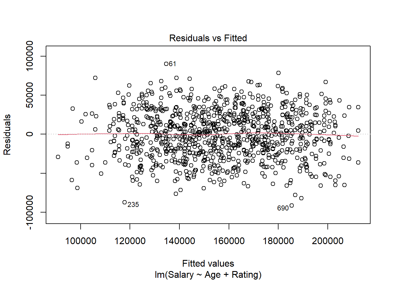
The residuals \(e_i\), also called the errors, are the observed (\(y_i\)) minus the predicted (\(\hat{y_i}\)) values for each row in our data set. The most basic plot is a residual versus fitted (predicted) value plot. This plot is easily created in R as shown below, and if the modeling assumptions are correct should show a random scatter of points. Note that we pass our regression model into the same plot() function we have seen before, but set the which argument to 1 in order to get a residual vs. fitted plot.
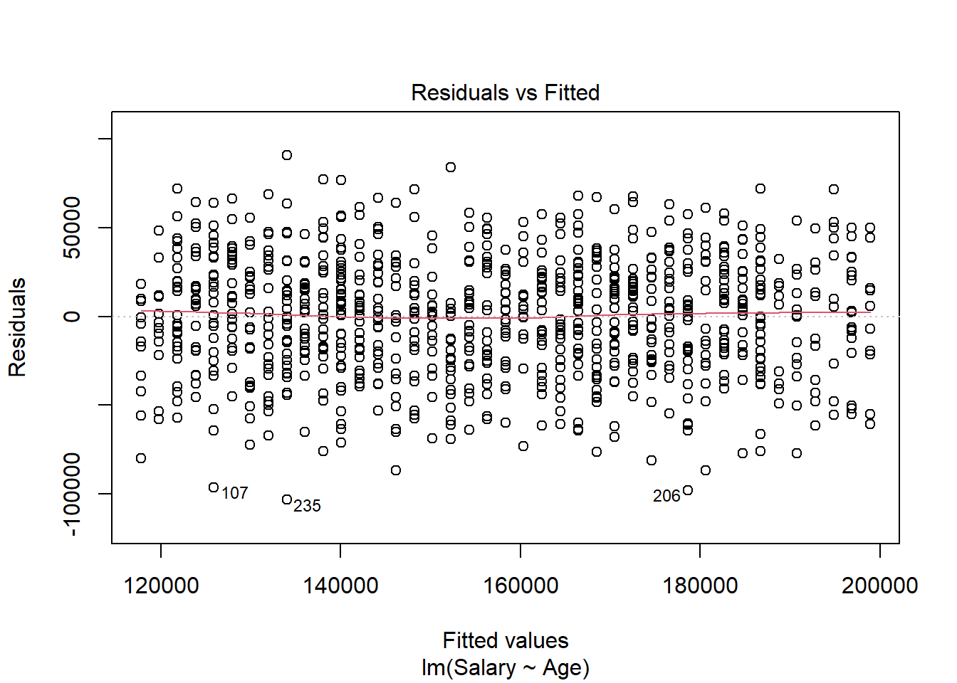
The red line shown in the plot is a local linear smooth used to capture the trend of the points. We see no relationship between the residuals and the fitted values, which must be true if the regression assumptions hold.
To contrast with the ideal plot, consider some simulated data of a non-linear relationship between \(X\) and \(Y\), which we don’t know so we fit a line. As the plots below indicate, there is an unusual relationship between the residuals and fitted values that would indicate we should investigate this model more fully.
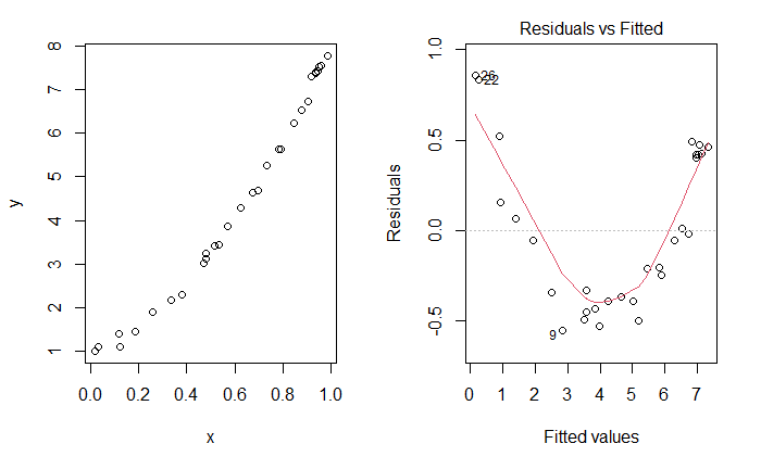
Figure 6.2: Unusual Residuals v. Fitted Plot.
The normality assumption of the noise in the model may be checked by either looking at a histogram or a qq-plot of the error terms. We can extract an atomic vector of the residuals from our model using the residuals() function:
residuals(fit)
By passing these residuals into hist(), we can observe the histogram of the residuals to check whether they are normally-distributed:
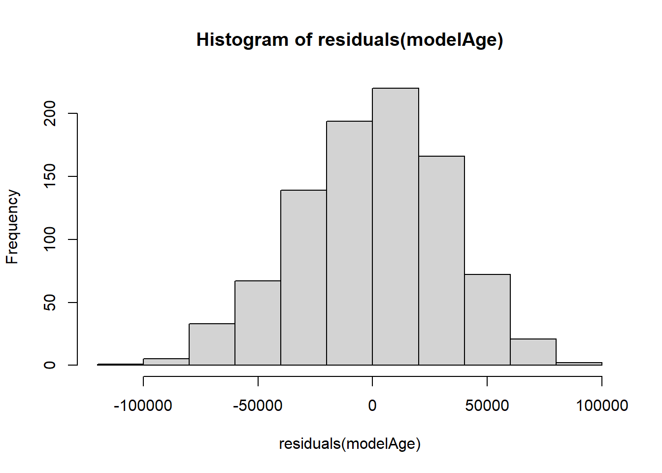
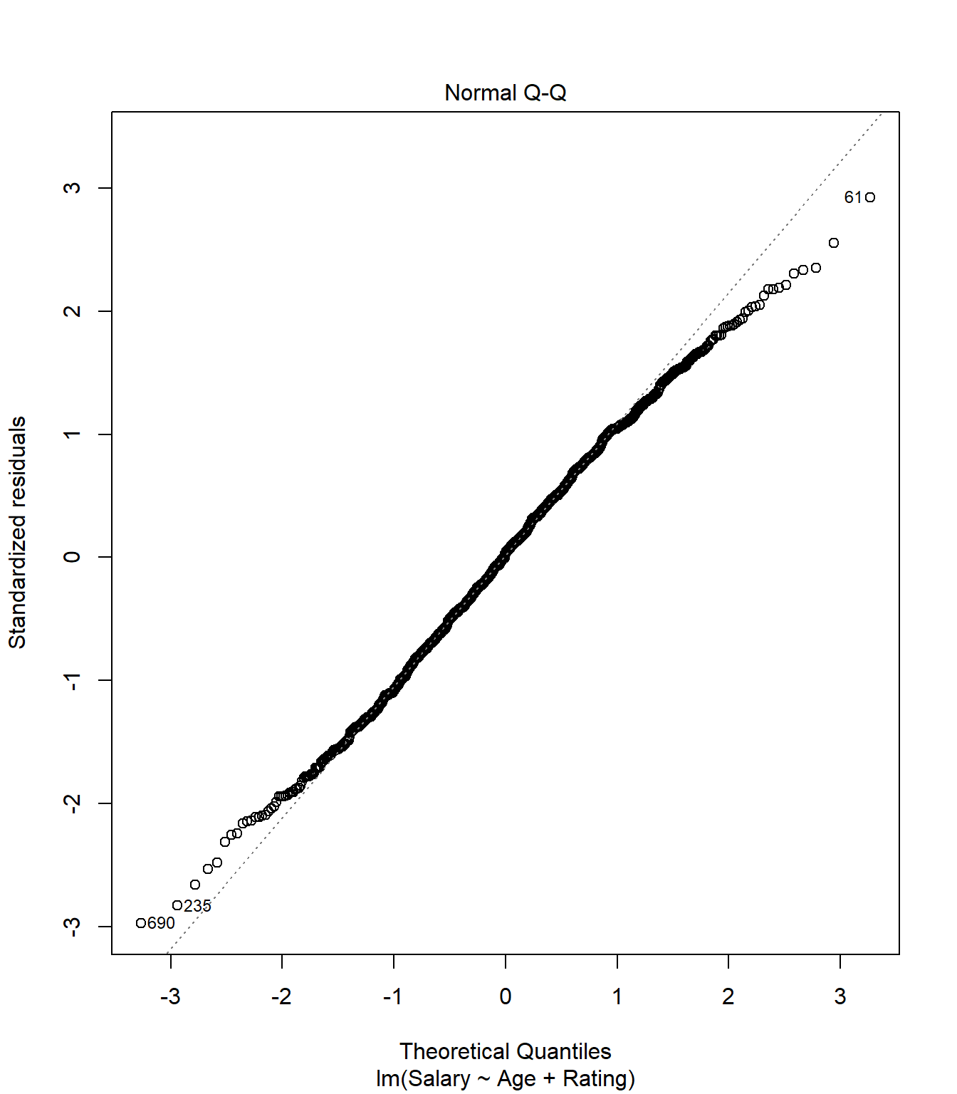
Based on this plot, the residuals of our model appear to be relatively normal. Another important diagnostic plot to look at is the qq-plot, which also helps us visually inspect whether our residuals are normally distributed. A qq-plot plots the residuals from our model against a straight line. If the plotted residuals fall mostly on the straight line, we conclude that they are most likely normally-distributed. If they deviate from the straight line, we conclude they might not be normally-distributed.
To create the qq-plot, we can pass our model into the plot() function and set the which parameter equal to 2:
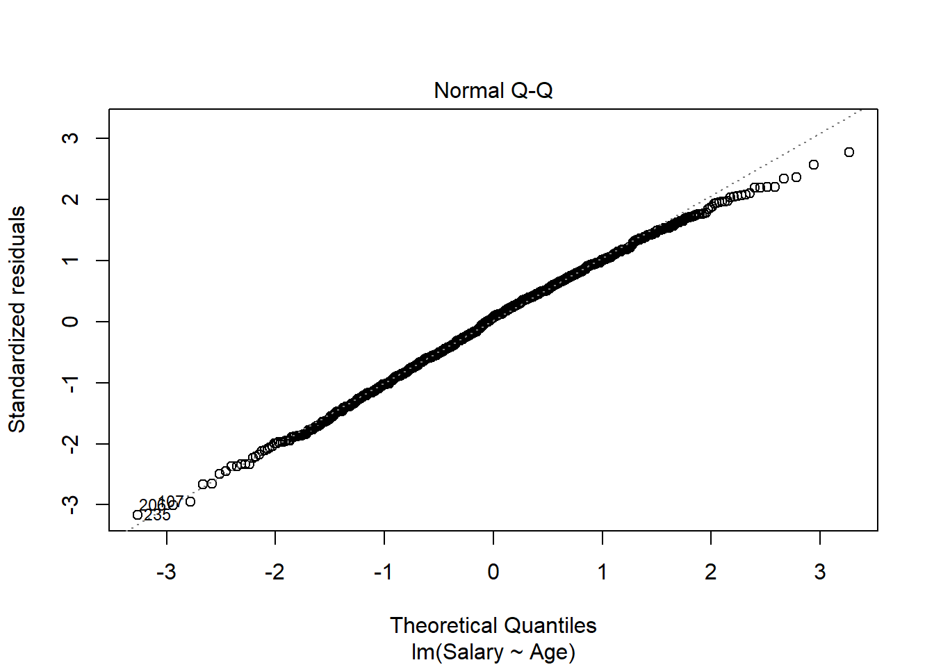
Consistent with the histogram of the residuals, the qq-plot shows that the residuals are approximately normal (i.e., they mostly fall on the straight line).
Always verify that the model residuals are normally distributed.
6.1.2 Multiple Linear Regression
In multiple linear regression we desire to model a dependent \(Y\) as a linear function of more than one explanatory variable. The assumed underlying relationship is:
\[Y = \beta_0 + \beta_1X_1 + \beta_2X_2 + \ldots + \beta_kX_k + \epsilon\]
The fundamental ideas of regression introduced for the simple linear regression model hold for multiple regression as well. In short, for multiple regression:
- Estimation is done by the method of least squares.
- Confidence intervals can be obtained for each coefficient.
- Hypothesis tests can be performed for each coefficient.
- \(R_a^2\) is a measure of how much variation in the \(y\) variable the \(x\) variables (together) explain.
- The errors are calculated as observed values minus predicted values.
- The noise in the system is assumed to be normally distributed, with a fixed variance that does not vary with \(x\).
- \(s_e\) is a measure of how accurate the predictions are.
The only main difference is in interpreting the estimated regression coefficients. In Latin the term ceteris paribus means “everything else (i.e., all other conditions) staying the same.” We apply this concept when we interpret regression coefficients in a multiple regression. For example, how do we interpret \(b_2\)? We would like to say that for a one unit change in \(x_2\), \(y\) changes by \(b_2\) (on average). But what happens to all the other variables in the model when we change \(x_2\)? To interpret the coefficient, we assume they remain constant. So we interpret \(b_k\) by saying that if \(x_k\) changes by one unit, then \(y\) changes by \(b_k\) on average assuming all other variables in the model remain constant.
As an example, let’s now model Salary from the employees data set as a function of both Age and Rating. We again use the lm() function, but now specify multiple explanatory variables in the regression formula:
lm(y ~ x1 + x2 + … + xp, data=df)
- Required arguments
y: The name of the dependent (\(Y\)) variable.x1,x2, …xp: The name of the first, second, and \(pth\) independent variables.data: The name of the data frame with they,x1,x2, andxpvariables.
##
## Call:
## lm(formula = Salary ~ Age + Rating, data = employees)
##
## Residuals:
##    Min     1Q Median     3Q    Max
## -91521 -21560    885  22729  90085
##
## Coefficients:
##             Estimate Std. Error t value             Pr(>|t|)
## (Intercept) 30505.51    5453.65   5.594         0.0000000294 ***
## Age          1966.05      92.83  21.180 < 0.0000000000000002 ***
## Rating       5604.08     530.60  10.562 < 0.0000000000000002 ***
## ---
## Signif. codes:  0 '***' 0.001 '**' 0.01 '*' 0.05 '.' 0.1 ' ' 1
##
## Residual standard error: 30830 on 917 degrees of freedom
##   (80 observations deleted due to missingness)
## Multiple R-squared:  0.3916, Adjusted R-squared:  0.3902
## F-statistic: 295.1 on 2 and 917 DF,  p-value: < 0.00000000000000022
Based on this output, our new estimated regression equation is:
\[predicted \;salary = \hat{y} = \$30505.51 + \$1966.05(Age) + \$5604.08(Rating)\]
We interpret the regression coefficients as follows:
- On average, employees who are zero years old and have a rating of zero make $30505.51. Clearly the intercept is not interpretable by itself but helps to anchor the line and give a baseline value for predictions.
- On average, salary goes up by $1966.05 for each additional year of age, assuming all other variables in the model are kept constant.
- On average, salary goes up by $5604.08 for each additional point in an employee’s rating, assuming all other variables in the model are kept constant.
6.1.2.1 The overall \(F\) test
If we look at the last line of the regression output above we see something called the F-statistic. This is an overall goodness of fit test that is used in multiple regression. This statistic is testing the null hypothesis that no explanatory variables are needed in the model. If we reject this test by having a small p-value (traditionally less than 0.05) we may conclude that we need at least one explanatory variable in the model. However, we are not told which one we need. Although this seems like a silly test, it is one that is very robust to model misspecification so we will usually look at it first when doing model building to make sure there is some explanatory power in the model.
6.1.2.2 Basic Diagnostic Plots
As we did with simple linear regression, we can examine diagnostic plots to see if the regression assumptions hold. The residuals versus fitted plot below has essentially a random scatter, indicating that there is no need to look for nonlinear relationships between the \(X\) variables and \(Y\).
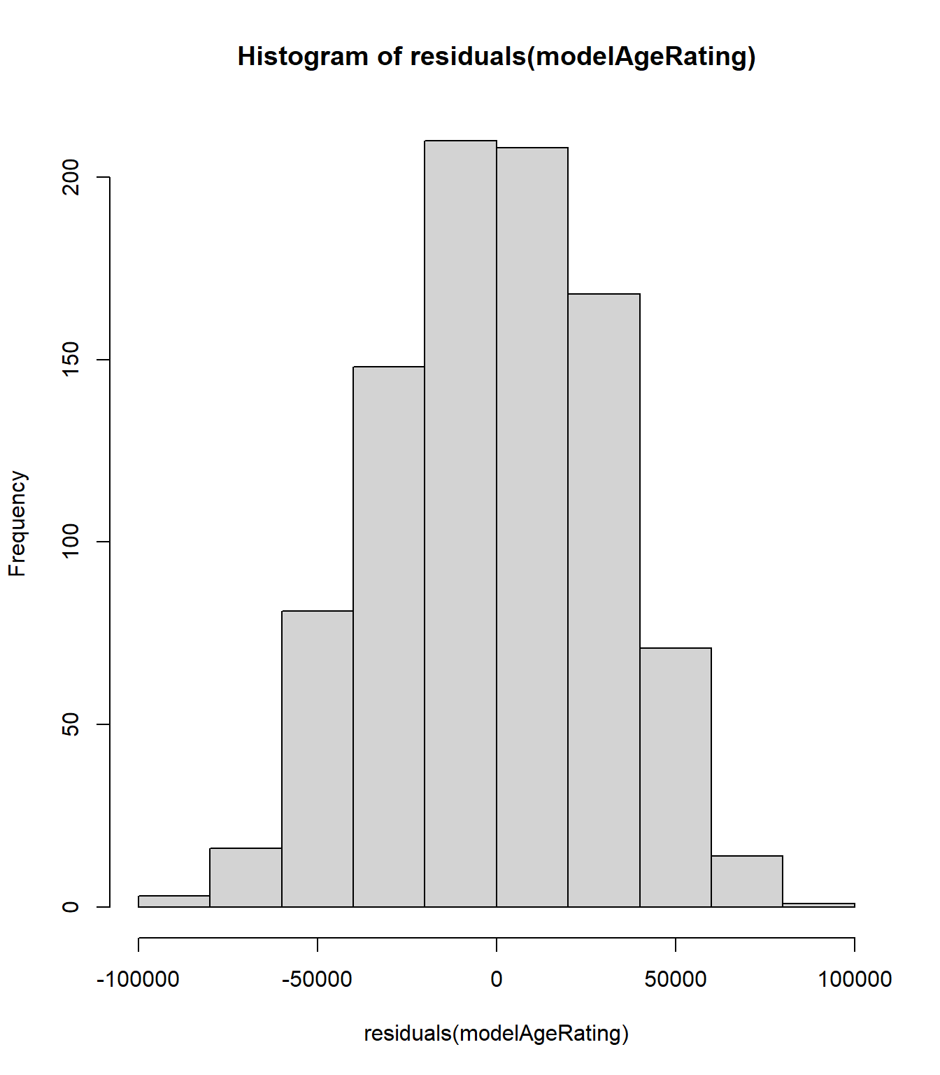
Additionally, a histogram and qq-plot of the residuals indicates that our new model errors are approximately normal.
6.1.3 Dummy Variables
So far we have been modeling Salary as a function of Age and Rating, which are both quantitative variables. However, there are also categorical variables in our data set that we might want to include in the model. For example, we might be interested in exploring whether there is a gender bias in our salary data. To do this, we need to somehow include Gender as an independent variable in our regression. However, this variable is not measured numerically; it takes on the values “Male” or “Female”. How, then, can we include it in our regression model?
To do this we need to create a dummy variable, or a binary, quantitative variable that is used to represent categorical data. Dummy variables use the numeric quantities 0 and 1 to represent the categories of interest. In our case our categorical variable is Gender, so our dummy needs to encode one of the genders as 0 and the other as 1. (Note that it is largely arbitrary which category we assign to 1 and which we assign to 0.) Let’s create a new variable in our data set called male_dummy, which equals 1 if the employee is male and 0 if the employee is female:
Now that we’ve created a dummy variable for gender, we can add it to our regression model:
##
## Call:
## lm(formula = Salary ~ Age + Rating + male_dummy, data = employees)
##
## Residuals:
##    Min     1Q Median     3Q    Max
## -91483 -21741    803  22130  85908
##
## Coefficients:
##             Estimate Std. Error t value             Pr(>|t|)
## (Intercept) 27047.67    5472.39   4.943          0.000000917 ***
## Age          1964.33      92.04  21.343 < 0.0000000000000002 ***
## Rating       5520.34     526.47  10.486 < 0.0000000000000002 ***
## male_dummy   8278.08    2017.04   4.104          0.000044214 ***
## ---
## Signif. codes:  0 '***' 0.001 '**' 0.01 '*' 0.05 '.' 0.1 ' ' 1
##
## Residual standard error: 30570 on 916 degrees of freedom
##   (80 observations deleted due to missingness)
## Multiple R-squared:  0.4025, Adjusted R-squared:  0.4006
## F-statistic: 205.7 on 3 and 916 DF,  p-value: < 0.00000000000000022
This produces the following estimated regression equation:
\[predicted \;salary = \hat{y} = \$27047.67 + \$1964.33(Age) + \$5520.34(Rating) + \$8278.08(male\_dummy)\]
The interpretation of the coefficients on Age and Rating are the same as before; for example, we would say that on average, salary goes up by $5520.34 for each additional point in an employee’s rating, assuming all other variables in the model are kept constant. However, a similar interpretation would not be possible for the coefficient on male_dummy, as this variable can only take on the values 0 and 1. Instead we interpret this coefficient as follows: on average, men at the company are paid $8278.08 more than women at the company, assuming all other variables in the model are kept constant. Because the p-value on this coefficient is quite small, we might conclude from these results that there does appear to be a gender bias in the company’s salary data.
To better understand the coefficient on the dummy variable, consider two employees, one male and one female. Assume that they are both 35, and both received an 8 in their last performance evaluation. For the male employee, our model would predict his salary to be:
\[\begin{aligned}predicted \;salary = \hat{y} & = \$27047.67 + \$1964.33(35) + \$5520.34(8) + \$8278.08(1) \\ & = \$139961.94 + \$8278.08(1) \\ & = \$148240.02\end{aligned}\]
Conversely, for the female employee, our model would predict her salary to be:
\[\begin{aligned}predicted \;salary = \hat{y} & = \$27047.67 + \$1964.33(35) + \$5520.34(8) + \$8278.08(0) \\ & = \$139961.94 + \$8278.08(0) \\ & = \$139961.94\end{aligned}\]
From this example we can see that when the other variables are held constant, the difference between the predicted salary for men and women is the value of the coefficient on our dummy variable.
In this example, we manually created a dummy variable for gender (called male_dummy) and used that variable in our model. However, this was not actually necessary - the lm() function automatically converts any categorical variables you include into dummy variables behind the scenes. If we specify our model as before but include Gender instead of male_dummy, we get the same results:
##
## Call:
## lm(formula = Salary ~ Age + Rating + Gender, data = employees)
##
## Residuals:
##    Min     1Q Median     3Q    Max
## -91483 -21741    803  22130  85908
##
## Coefficients:
##             Estimate Std. Error t value             Pr(>|t|)
## (Intercept) 27047.67    5472.39   4.943          0.000000917 ***
## Age          1964.33      92.04  21.343 < 0.0000000000000002 ***
## Rating       5520.34     526.47  10.486 < 0.0000000000000002 ***
## GenderMale   8278.08    2017.04   4.104          0.000044214 ***
## ---
## Signif. codes:  0 '***' 0.001 '**' 0.01 '*' 0.05 '.' 0.1 ' ' 1
##
## Residual standard error: 30570 on 916 degrees of freedom
##   (80 observations deleted due to missingness)
## Multiple R-squared:  0.4025, Adjusted R-squared:  0.4006
## F-statistic: 205.7 on 3 and 916 DF,  p-value: < 0.00000000000000022
Dummy variables are relatively straightforward for binary categorical variables such as Gender. But what about a variable like Degree, which can take on several different values (“High School”, “Associate’s”, “Bachelor’s”, “Master’s”, and “Ph.D”)? It might be natural to assume that you could just assign a unique integer to each category. In other words, our dummy for degree could represent “High School” as 0, “Associate’s” as 1, “Bachelor’s” as 2, “Master’s” as 3, and “Ph.D” as 4. However, this method of coding categorical variables is problematic. First, it implies an ordering to the categories that may not be correct. There might be an ordering to Degree, but consider the Division variable; there is no inherent ordering to the divisions of a company, so any ordering implied by a dummy variable would be arbitrary. Second, this method of coding implies a fixed difference between each category. There is no reason to believe that the difference between an associate’s and a bachelor’s is the same as the difference between a bachelor’s and a master’s, for example.
How, then, do we incorporate multinomial categorical variables into our regression model? The answer is by creating separate 0 / 1 dummy variables for each of the variable’s categories. For example, we will need one dummy variable (DegreeAssociate's) that equals 1 for observations where Degree equals “Associate’s”, and 0 if not. We will need another dummy variable (DegreeBachelor's) that equals 1 for observations where Degree equals “Bachelor’s” and 0 if not, and so on. The table below shows how all possible values of Degree can be represented through four binary dummy variables:
| Degree | DegreeAssociate’s | DegreeBachelor’s | DegreeMaster’s | DegreePh.D |
|---|---|---|---|---|
| High School | 0 | 0 | 0 | 0 |
| Associate’s | 1 | 0 | 0 | 0 |
| Bachelor’s | 0 | 1 | 0 | 0 |
| Master’s | 0 | 0 | 1 | 0 |
| Ph.D | 0 | 0 | 0 | 1 |
Note that we do not need a fifth dummy variable to represent the “High School” category. This is because this information is already implicitly captured in the other four dummy variables; if DegreeAssociate's, DegreeBachelor's, DegreeMaster's, and DegreePh.D all equal zero, we know the employee must hold a high school diploma, so there is no need for an additional DegreeHighSchool variable. In general, a \(k\)-category variable can be represented with \(k-1\) dummy variables.
For regression modeling, categorical variables that take on \(k\) values must be converted into \(k-1\) binary dummy variables.
As noted above, the lm() command automatically creates dummy variables behind the scenes, so we can simply include Degree in our call to lm():
##
## Call:
## lm(formula = Salary ~ Age + Rating + Gender + Degree, data = employees)
##
## Residuals:
##    Min     1Q Median     3Q    Max
## -64403 -16227    352  15917  70513
##
## Coefficients:
##                    Estimate Std. Error t value             Pr(>|t|)
## (Intercept)           4.427   4502.240   0.001             0.999216
## Age                2006.083     70.078  28.627 < 0.0000000000000002 ***
## Rating             5181.073    401.489  12.905 < 0.0000000000000002 ***
## GenderMale         8220.111   1532.334   5.364          0.000000103 ***
## DegreeAssociate's  9477.556   2444.091   3.878             0.000113 ***
## DegreeBachelor's  33065.808   2426.033  13.630 < 0.0000000000000002 ***
## DegreeMaster's    40688.574   2410.054  16.883 < 0.0000000000000002 ***
## DegreePh.D        53730.605   2408.267  22.311 < 0.0000000000000002 ***
## ---
## Signif. codes:  0 '***' 0.001 '**' 0.01 '*' 0.05 '.' 0.1 ' ' 1
##
## Residual standard error: 23220 on 912 degrees of freedom
##   (80 observations deleted due to missingness)
## Multiple R-squared:  0.6568, Adjusted R-squared:  0.6541
## F-statistic: 249.3 on 7 and 912 DF,  p-value: < 0.00000000000000022
To interpret the coefficients on the dummy variables for degree, we must first acknowledge that they are all relative to the implicit baseline category, “High School”. The baseline (or reference) category is the one that is not given its own dummy variable; in this case we do not have a separate dummy for “High School”, so it is our baseline. With this in mind, we interpret the coefficients on our dummy variables as follows:
- On average, employees with an Associate’s degree are paid $9477.56 more than employees with a high school diploma, assuming all other variables in the model are kept constant.
- On average, employees with a Bachelor’s degree are paid $33065.81 more than employees with a high school diploma, assuming all other variables in the model are kept constant.
- On average, employees with an Master’s degree are paid $40688.57 more than employees with a high school diploma, assuming all other variables in the model are kept constant.
- On average, employees with a Ph.D are paid $53730.61 more than employees with a high school diploma, assuming all other variables in the model are kept constant.
6.1.4 Transformations
[In Progress]
6.1.5 Interactions
[In Progress]
6.1.6 Model Diagnostics
[In Progress]
6.1.6.1 Testing for Non-Linearity
[In Progress]
6.1.6.2 Multicollinearity
[In Progress]
6.1.6.3 Normality of Residuals
[In Progress]
6.1.6.4 Heteroskedasticity
[In Progress]
6.2 Logistic Regression
The linear regression model described in the previous section allows one to model a continuous dependent variable as a function of one or more independent variables. However, what if we would instead like to model a categorical outcome? Logistic regression (or the logit model) was developed by statistician David Cox in 1958 and is a regression model where the response variable \(Y\) is categorical. Logistic regression allows us to estimate the probability of a categorical response based on one or more predictor variables (\(X\)). In this section we will cover the case when \(Y\) is binary — that is, where it can take only two values, 0 and 1, which represent outcomes such as pass/fail, win/lose, alive/dead, healthy/sick, etc.
Cases where the dependent variable has more than two outcome categories may be analyzed with multinomial logistic regression, or, if the multiple categories are ordered, ordinal logistic regression, although we will not cover these methods here.
6.2.1 Why Not Linear Regression?
At this point, a natural question might be why one cannot use linear regression to model categorical outcomes. To understand why, let’s look at an example. We have a data set related to a telephone marketing campaign of a Portuguese banking institution. Suppose we would like to model the likelihood that a phone call recipient will make a term deposit at the bank. The data is saved in a data frame called deposit, and the first few observations are shown below:
| age | marital | education | default | housing | loan | contact | duration | campaign | previous | poutcome | subscription |
|---|---|---|---|---|---|---|---|---|---|---|---|
| 30 | married | primary | no | no | no | cellular | 79 | 1 | 0 | unknown | 0 |
| 33 | married | secondary | no | yes | yes | cellular | 220 | 1 | 4 | failure | 0 |
| 35 | single | tertiary | no | yes | no | cellular | 185 | 1 | 1 | failure | 0 |
| 30 | married | tertiary | no | yes | yes | unknown | 199 | 4 | 0 | unknown | 0 |
| 59 | married | secondary | no | yes | no | unknown | 226 | 1 | 0 | unknown | 0 |
| 35 | single | tertiary | no | no | no | cellular | 141 | 2 | 3 | failure | 0 |
These variables are defined as follows:
age: The age of the person contacted.marital: The marital status of the person contacted.education: The education level of the person contacted.default: Whether the person contacted has credit in default.housing: Whether the person contacted has a housing loan.loan: Whether the person contacted has a personal loan.contact: How the person was contacted (cellularortelephone).duration: The duration of the contact, in seconds.campaign: The number of contacts performed during this campaign for this client.previous: The number of contacts performed before this campaign for this client.poutcome: The outcome of the previous marketing campaign (failure,nonexistent, orsuccess).subscription: Whether the person contacted made a term deposit (1if the person made a deposit and0if not).
Let’s try using linear regression to model subscription as a function of duration:
##
## Call:
## lm(formula = subscription ~ duration, data = deposit)
##
## Residuals:
##      Min       1Q   Median       3Q      Max
## -1.47629 -0.11329 -0.05758 -0.01963  1.00009
##
## Coefficients:
##                Estimate  Std. Error t value            Pr(>|t|)
## (Intercept) -0.01487918  0.00620255  -2.399              0.0165 *
## duration     0.00049295  0.00001675  29.436 <0.0000000000000002 ***
## ---
## Signif. codes:  0 '***' 0.001 '**' 0.01 '*' 0.05 '.' 0.1 ' ' 1
##
## Residual standard error: 0.2926 on 4519 degrees of freedom
## Multiple R-squared:  0.1609, Adjusted R-squared:  0.1607
## F-statistic: 866.5 on 1 and 4519 DF,  p-value: < 0.00000000000000022
Based on this output, our estimated regression equation is:
\[predicted \;subscription = \hat{y} = -0.01488 + 0.00049(duration)\]
If we plot this line on top of our data, we can start to see the problem:
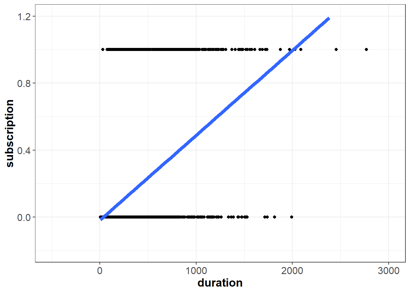
Our independent variable subscription can only take on two possible values, 0 and 1. However, the line we fit is not bounded between zero and one. If duration equals 2,500 seconds, for example, the model would predict a value greater than one:
\[\begin{aligned}predicted \;subscription = \hat{y} & \approx -0.01488 + 0.00049(2500) \\ & \approx -0.01 + 1.23 \\ & \approx 1.22\end{aligned}\]
A negative value of duration does not make sense in this context, but in principle the same problem applies in the opposite direction - for small values of \(X\), the linear model might predict outcomes less than zero. To overcome this issue, logistic regression models the dependent variable \(Y\) according to the logistic function, which is bounded between zero and one.
6.2.2 Simple Logistic Regression
Instead of modeling the response variable (\(Y\)) directly, logistic regression uses independent (\(X\)) variables to model the probability that \(Y\) equals the outcome of interest. In other words, logistic regression allows us to model \(P(Y = 1 | X)\), or the probability that \(Y\) equals one given \(X\). To do this, we need a mathematical function that provides predictions between zero and one for all possible values of \(X\). There are many functions that meet this description, but for logistic regression we use the logistic function and assume the following relationship:
\[P(Y = 1 | X) = \frac{e^{\beta_0+\beta_1X}}{1+e^{\beta_0+\beta_1X}}\] As with linear regression, our goal is to find estimates of \(\beta_0\) and \(\beta_1\) using our observed data. Whereas linear regression does this using the method of least squares, logistic regression calculates sample estimates of \(\beta_0\) and \(\beta_1\) using a method known as maximum likelihood estimation (MLE). We will not describe MLE in detail, but it essentially uses the sample data to find estimates of \(\beta_0\) and \(\beta_1\) such that the model’s predicted probability is high when \(Y\) actually equals one and low when \(Y\) actually equals zero.
We can fit a logistic regression model in R with the glm() command (the glm stands for general linear model). This function uses the following syntax:
glm(y ~ x, data=df, family=“binomial”)
- Required arguments
y: The name of the dependent (\(Y\)) variable.x: The name of the independent (\(X\)) variable.data: The name of the data frame with theyandxvariables.family: The type of model we would like to fit; for logistic regression, we set this equal to"binomial"because we are modeling a binomial process (i.e., one with two possible outcomes).
As with linear regression, we can fit a logistic regression to our data and then use summary() to obtain detailed information about the model:
##
## Call:
## glm(formula = subscription ~ duration, family = "binomial", data = deposit)
##
## Deviance Residuals:
##     Min       1Q   Median       3Q      Max
## -3.8683  -0.4303  -0.3548  -0.3106   2.5264
##
## Coefficients:
##               Estimate Std. Error z value            Pr(>|z|)
## (Intercept) -3.2559346  0.0845767  -38.50 <0.0000000000000002 ***
## duration     0.0035496  0.0001714   20.71 <0.0000000000000002 ***
## ---
## Signif. codes:  0 '***' 0.001 '**' 0.01 '*' 0.05 '.' 0.1 ' ' 1
##
## (Dispersion parameter for binomial family taken to be 1)
##
##     Null deviance: 3231.0  on 4520  degrees of freedom
## Residual deviance: 2701.8  on 4519  degrees of freedom
## AIC: 2705.8
##
## Number of Fisher Scoring iterations: 5
Based on this output, our estimated regression equation is:
\[\begin{aligned}predicted \;probability = \hat{p}(y=1) = \frac{e^{-3.25593+0.00355(duration)}}{1+e^{-3.25593+0.00355(duration)}}\end{aligned}\]
If we plot this line on top of our data, we can see how logistic regression suits the problem better than linear regression. Because the logistic function is bounded between zero and one, we see the characteristic “s-shape” curve:
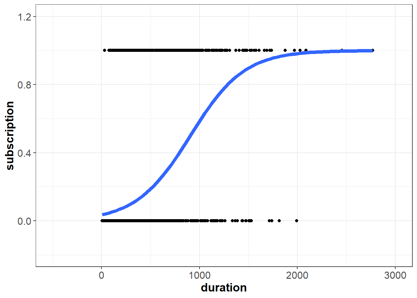
Now if duration equals 2,500 seconds, the model’s prediction does not exceed one:
\[\begin{aligned}predicted \;probability = \hat{p}(y=1) & \approx \frac{e^{-3.25593+0.00355(2500)}}{1+e^{-3.25593+0.00355(2500)}} \\ & \approx \frac{275.3237478}{276.3237478} \\ & \approx 0.9963811 \end{aligned}\]
We can also use the model to make predictions with the predict() function. Note that for logistic regression, we need to include type="response". This ensures that predict() returns the prediction as a probability between zero and one (as opposed to the log-odds form).
##         1
## 0.9963811
Because the logistic regression models a non-linear relationship, we cannot interpret the model coefficients as we did with linear regression. Instead, we interpret the coefficient on a continuous \(X\) as follows:
If \(b_1>0\), a one unit increase in the predictor corresponds to an increase in the probability that \(y = 1\). Note that we don’t specify the amount of the increase, as this is not as straight forward as linear regression where the amount is the value of the coefficient.
If \(b_1<0\), a one unit increase in the predictor corresponds to a decrease in the probability that \(y = 1\). Again, note that we don’t specify the amount of the decrease.
Using this guideline, we can interpret the \(b_1\) coefficient in our model as follows:
- Because \(b_1\) is greater than zero, a one-unit increase in
durationcorresponds to an increase in the probability that the contacted person makes a deposit.
Now instead of a continuous \(X\) like duration, let’s use the categorical \(X\) variable, loan. As a reminder, glm() automatically converts categorical variables to dummy variables behind the scenes, so we can simply include loan in our call to glm():
depositLogDummy <- glm(subscription ~ loan, data=deposit, family="binomial")
summary(depositLogDummy)
##
## Call:
## glm(formula = subscription ~ loan, family = "binomial", data = deposit)
##
## Deviance Residuals:
## Min 1Q Median 3Q Max
## -0.5163 -0.5163 -0.5163 -0.3585 2.3567
##
## Coefficients:
## Estimate Std. Error z value Pr(>|z|)
## (Intercept) -1.94770 0.04889 -39.837 < 0.0000000000000002 ***
## loanyes -0.76499 0.16489 -4.639 0.00000349 ***
## ---
## Signif. codes: 0 '***' 0.001 '**' 0.01 '*' 0.05 '.' 0.1 ' ' 1
##
## (Dispersion parameter for binomial family taken to be 1)
##
## Null deviance: 3231.0 on 4520 degrees of freedom
## Residual deviance: 3205.2 on 4519 degrees of freedom
## AIC: 3209.2
##
## Number of Fisher Scoring iterations: 5If \(X\) is a dummy variable, we interpret the coefficient as follows:
If \(b_1>0\), observations where the dummy equals one have a greater probability that \(y = 1\).
If \(b_1<0\), observations where the dummy equals one have a lower probability that \(y = 1\).
Applying this to our output, we interpret the negative coefficient on loanyes as follows:
- On average, contacted persons who have a personal loan (i.e.,
loanyes = 1) have a lower probability of making a deposit than contacted persons who do not have a personal loan.
6.2.3 Multiple Logistic Regression
Much like linear regression, logistic regression can include multiple independent (\(X\)) variables. When there is more than one \(X\), we assume the following relationship:
\[P(Y = 1 | X) = \frac{e^{\beta_0+\beta_1X_1+\beta_2X_2+...+\beta_pX_p}}{1+e^{\beta_0+\beta_1X_1+\beta_2X_2+...+\beta_pX_p}}\]
Below we fit a multiple logistic regression using several of the independent variables in our data set:
depositLogMultiple <- glm(subscription ~ duration + campaign + loan + marital,
                          data=deposit, family="binomial")
summary(depositLogMultiple)
##
## Call:
## glm(formula = subscription ~ duration + campaign + loan + marital,
## family = "binomial", data = deposit)
##
## Deviance Residuals:
## Min 1Q Median 3Q Max
## -3.9111 -0.4469 -0.3560 -0.2684 2.7765
##
## Coefficients:
## Estimate Std. Error z value Pr(>|z|)
## (Intercept) -2.6923460 0.1629547 -16.522 < 0.0000000000000002 ***
## duration 0.0036105 0.0001753 20.594 < 0.0000000000000002 ***
## campaign -0.0995488 0.0256961 -3.874 0.000107 ***
## loanyes -0.8927075 0.1821953 -4.900 0.00000096 ***
## maritalmarried -0.3825457 0.1547694 -2.472 0.013447 *
## maritalsingle -0.0539759 0.1668874 -0.323 0.746372
## ---
## Signif. codes: 0 '***' 0.001 '**' 0.01 '*' 0.05 '.' 0.1 ' ' 1
##
## (Dispersion parameter for binomial family taken to be 1)
##
## Null deviance: 3231 on 4520 degrees of freedom
## Residual deviance: 2641 on 4515 degrees of freedom
## AIC: 2653
##
## Number of Fisher Scoring iterations: 6We interpret these estimated coefficients as follows:
- On average, a one-unit increase in
durationcorresponds to an increase in the probability that the contacted person makes a deposit, assuming all other variables in the model are kept constant. - On average, a one-unit increase in
campaigncorresponds to a decrease in the probability that the contacted person makes a deposit, assuming all other variables in the model are kept constant. - On average, contacted persons with a personal loan are less likely to make a deposit than contacted persons without a personal loan, assuming all other variables in the model are kept constant.
- On average, contacted persons who are married are less likely to make a deposit than contacted persons who are divorced, assuming all other variables in the model are kept constant. Note that
maritalcan take on three possible values (divorced,married, andsingle), sodivorcedis our baseline because the model created explicit dummies for the other two categories (maritalmarriedandmaritalsingle). - On average, contacted persons who are single are less likely to make a deposit than contacted persons who are divorced, assuming all other variables in the model are kept constant. However, the p-value on this coefficient is quite large, so we cannot conclude that this difference is statistically significant.
6.3 Regression Model Building
[In Progress]
6.3.0.1 All Subsets
[In Progress]
6.3.0.2 Akaike Information Criterion (AIC)
[In Progress]
6.3.0.3 Stepwise Regression
[In Progress]