B Quick Start
B.1 Linear Regression
See also Section 6.1.
Suppose we have a data frame called housing with real estate transaction data from Saratoga Springs, New York (ADD source: https://dasl.datadescription.com/datafile/saratoga-house-prices/). The first few observations of this data set are shown below.
| Price | Baths | Bedrooms | Fireplace | Acres | Age |
|---|---|---|---|---|---|
| 142.212 | 1.0 | 3 | 0 | 2.00 | 133 |
| 134.865 | 1.5 | 3 | 1 | 0.38 | 14 |
| 118.007 | 2.0 | 3 | 1 | 0.96 | 15 |
| 138.297 | 1.0 | 2 | 1 | 0.48 | 49 |
| 129.470 | 1.0 | 3 | 1 | 1.84 | 29 |
| 206.512 | 2.0 | 3 | 0 | 0.98 | 10 |
These variables are defined as follows:
Price: The sales price of a home in thousands of dollars.Baths: The number of bathrooms in the home.Bedrooms: The number of bedrooms in the home.Fireplace: Whether the home has a fireplace.Acres: The lot size in acres.Age: The age of the home in years.
We can fit a regression with Price as the dependent (\(Y\)) variable using the lm() function as follows:
Then we can apply the summary() function to fit to get a summary of our model:
##
## Call:
## lm(formula = Price ~ Baths + Bedrooms + Fireplace + Acres + Age,
##     data = housing)
##
## Residuals:
##     Min      1Q  Median      3Q     Max
## -141.47  -33.43   -6.11   19.78  470.00
##
## Coefficients:
##              Estimate Std. Error t value             Pr(>|t|)
## (Intercept) -27.17190    8.61390  -3.154             0.001654 **
## Baths        65.38343    3.78293  17.284 < 0.0000000000000002 ***
## Bedrooms     16.92751    2.91667   5.804        0.00000000857 ***
## Fireplace    21.12512    4.27226   4.945        0.00000088638 ***
## Acres         8.78877    2.37834   3.695             0.000231 ***
## Age          -0.04538    0.05945  -0.763             0.445458
## ---
## Signif. codes:  0 '***' 0.001 '**' 0.01 '*' 0.05 '.' 0.1 ' ' 1
##
## Residual standard error: 60.55 on 1057 degrees of freedom
## Multiple R-squared:  0.4887, Adjusted R-squared:  0.4863
## F-statistic: 202.1 on 5 and 1057 DF,  p-value: < 0.00000000000000022
We can apply confint() to fit() to get a 95% confidence interval for each of the coefficients of our model:
##                   2.5 %       97.5 %
## (Intercept) -44.0741786 -10.26961652
## Baths        57.9605197  72.80634988
## Bedrooms     11.2043862  22.65062633
## Fireplace    12.7420535  29.50819039
## Acres         4.1219695  13.45558042
## Age          -0.1620358   0.07127757
Finally, to check that our error terms are normally-distributed, we can create a qq-plot by applying the plot() function with which=2 as a parameter:
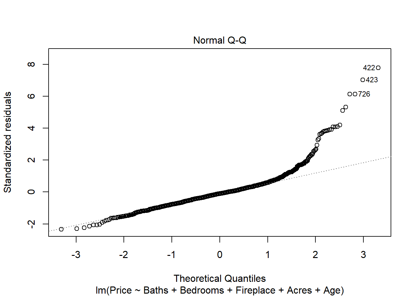
This qq-plot is problematic, as the right-hand side shows unusual tail behavior. This is likely because Price is positively-skewed; there are a handful of “outlier” houses that are very expensive. To address this, we could try fitting a new regression where we model the log of Price as our independent variable:
fitLog <- lm(log(Price) ~ Baths + Bedrooms + Fireplace + Acres + Age, data=housing)
plot(fitLog, which=2)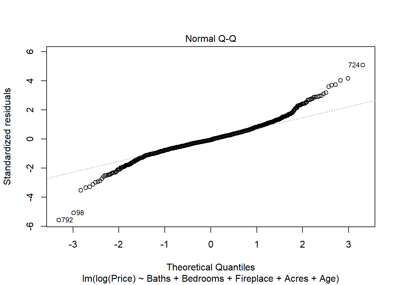
B.2 Estimating \(\beta\) of a Stock
To estimate the “beta” (\(\beta\)) of a stock:
- Load the
quantmodpackage. - Use the
getSymbols()function to pull the historical returns data for a particular stock over a given period. - Use
getSymbols()to pull the S&P 500 market returns data for the same time period. - Extract the returns from the objects created in steps 2 & 3.
- Use
lm()to regress the market returns onto the stock returns.
Following these steps, let’s calculate an estimate for the five-year monthly \(\beta\) on Disney at the time of writing (May 4, 2021). Note that “DIS” is the ticker for Disney and “SPY” is the ticker for the S&P 500.
# Step 1
library(quantmod)

# Step 2
DIS <- getSymbols("DIS", from="2016-05-04", to="2021-05-04", auto.assign=FALSE)

# Step 3
SPY <- getSymbols("SPY", from="2016-05-04", to="2021-05-04", auto.assign=FALSE)

# Step 4
disReturns <- monthlyReturn(Ad(DIS))
spyReturns <- monthlyReturn(Ad(SPY))

# Step 5
fit <- lm(disReturns ~ spyReturns)
summary(fit)
##
## Call:
## lm(formula = disReturns ~ spyReturns)
##
## Residuals:
## Min 1Q Median 3Q Max
## -0.07951 -0.04642 -0.01340 0.03205 0.18854
##
## Coefficients:
## Estimate Std. Error t value Pr(>|t|)
## (Intercept) -0.003560 0.007992 -0.445 0.658
## spyReturns 1.190923 0.178991 6.654 0.0000000104 ***
## ---
## Signif. codes: 0 '***' 0.001 '**' 0.01 '*' 0.05 '.' 0.1 ' ' 1
##
## Residual standard error: 0.05917 on 59 degrees of freedom
## Multiple R-squared: 0.4287, Adjusted R-squared: 0.419
## F-statistic: 44.27 on 1 and 59 DF, p-value: 0.00000001041Of course, it is important to note the 95% confidence interval on our estimate of \(\beta\), which we can get using confint():
##                   2.5 %     97.5 %
## (Intercept) -0.01955258 0.01243257
## spyReturns   0.83276270 1.54908236