Chapter 7 Causal Inference

Causal inference is a vast field that seeks to address questions relating causes to effects. We more formally define causal inference as the study of how a treatment (i.e., action or intervention) affects outcomes of interest relative to an alternate treatment. Often, one of the treatments represents a baseline or status quo: it is then called a control. Academics have used causal reasoning for over a century to establish many scientific findings we now consider as facts. In the past decade, there has been a rapid increase in the adoption of causal thinking by firms, and it is now an integral part of data science. Causal inference can be used to answer such questions as:

What is the effect on the throughput time (outcome) of introducing a new drill to a production line (treatment) relative to the current process (control)?
What is the effect of changing the text on the landing page’s button (treatment) on the clickthrough rate (outcome), relative to the current text (control)?
Which of two hospital admission processess (treatment 1 vs treatment 2) leads to the better health results (outcome)?

The most reliable way to establish causal relationships is to run a randomized experiment. Different fields have different names for these, including A/B tests, clinical trials, randomized control trials, etc… but basically, a randomized experiment involves randomly assigning subjects (e.g., customers, divisions, companies) to either receive a treatment or a control intervention. The effectiveness of the treatment is then assessed by contrasting the outcomes of the treated subjects to the outcomes of the control subjects.

The simple idea of running experiments has had a profound impact on how managers make decisions, as it allows them to discern their customers’ preferences, evaluate their initiatives, and ultimately test their hypotheses. Experimentation is now an integral part of the product development process at most technology companies. It is increasingly being adopted by non-technology companies as well, as they recognize that experimentation allows managers to continuously challenge their working hypotheses and perform pivots that ultimately lead to better innovations.

Unfortunately, we cannot always run experiments because of ethical concerns, high costs, or an inability to control the random assignment directly. Luckily, this is a challenge that academics have grappled with for a long time, and they have developed many different strategies for identifying causal effects from non-experimental (i.e., observational) data. For example, we know that smoking causes cancer even though no one ever ran a randomized experiment to measure the effect of smoking. However, it is important to understand that causal claims from observational data are inherently less reliable than claims derived from experimental evidence and can be subject to severe biases.

7.1 Observational Studies

The vast majority of statistics courses begin and end with the premise that correlation is not causation (see Section 4.1.1.1). But they rarely explain why we can not directly assume that correlation is not causation.

Let’s consider a simple example. Imagine you are working as a data scientist for Musicfi, a firm that offers on-demand music streaming services. To keep things simple, let’s assume the firm has two account types: a free account and a premium account. Musicfi’s main measure of customer engagement is the total streaming minutes that measure how many minutes each customer spent on the service per day. As a data scientist, you want to understand your customers, so you decide to perform a simple analysis that compares the total streaming minutes across the two account types. To put this in causal terms:

Our treatment is having a premium account
Our control is having a free account
Our outcome is total streaming minutes

Suppose we have a random sample of 500 customers, stored in a data frame called musicfi:

head(musicfi)

##   Age AccountType StreamingMinutes
## 1  33     Premium               63
## 2  38     Premium               61
## 3  24        Free               82
## 4  28     Premium               72
## 5  61     Premium               38
## 6  33        Free               71

First, let’s create a side-by-side boxplot that compares the StreamingMinutes of free and premium customers:

boxplot(musicfi$StreamingMinutes ~ musicfi$AccountType, 
        ylab = "Streaming Minutes", xlab = "Treatment")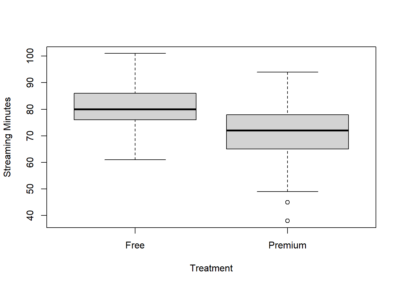

From the figure, we can see that the customers with premium accounts had lower total streaming minutes than customers with free accounts! The average in the premium group was 71 minutes compared to 80 minutes in the free group, meaning that (on average) customers with a premium account listened to less music! We can use a t-test to check if this observed difference is statistically significant:

t.test(musicfi$StreamingMinutes ~ musicfi$AccountType)

## 
##  Welch Two Sample t-test
## 
## data:  musicfi$StreamingMinutes by musicfi$AccountType
## t = 11.774, df = 444.24, p-value < 0.00000000000000022
## alternative hypothesis: true difference in means is not equal to 0
## 95 percent confidence interval:
##   7.52599 10.54174
## sample estimates:
##    mean in group Free mean in group Premium 
##              80.42205              71.38819

Suppose we take the above results at face value. In that case, we might incorrectly conclude that having a premium account reduces customer engagement. But this seems unlikely! Our general understanding suggests that buying a premium account should have the opposite effect. So what’s going on? Well, we are likely falling victim to what is often called selection bias. Selection bias occurs when the treatment group is systematically different from the control group before the treatment has occurred, making it hard to disentangle differences due to the treatment from those due to the systematic difference between the two groups.

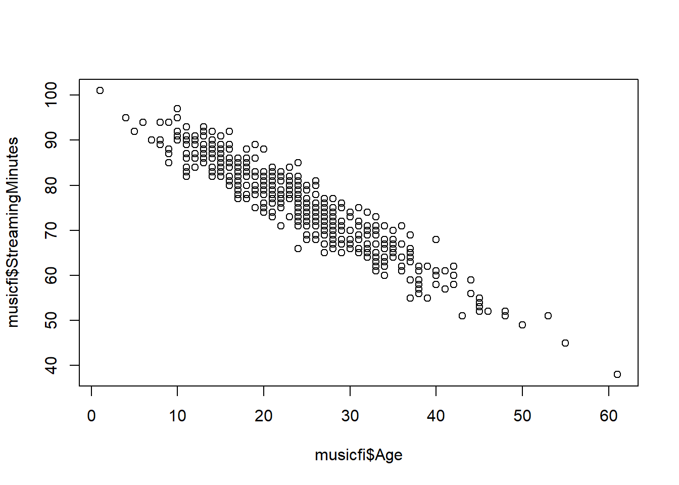
Mathematically, we can model selection bias as a third variable—often called a confounding variable—associated with both a unit’s propensity to receive the treatment and that unit’s outcome. In our Musicfi example, this variable could be the age of the customer: younger customers tend to listen to more music and are less likely to purchase a premium account. Therefore, the age variable is a confounding variable as it limits our ability to draw causal inferences.

To see this, we can compare how age is related to total streaming minutes and the account type. First, let’s create a scatter plot of age and streaming minutes:

plot(musicfi$Age, musicfi$StreamingMinutes)

If we wanted to adjust for the age variable (assuming it is observed), we could run a linear regression with both AccountType and Age as independent variables:

summary(lm(StreamingMinutes ~ AccountType + Age, data=musicfi))

## 
## Call:
## lm(formula = StreamingMinutes ~ AccountType + Age, data = musicfi)
## 
## Residuals:
##     Min      1Q  Median      3Q     Max 
## -9.1032 -2.2259  0.0901  2.0055  8.6514 
## 
## Coefficients:
##                     Estimate Std. Error t value             Pr(>|t|)    
## (Intercept)        100.57573    0.41028 245.138 < 0.0000000000000002 ***
## AccountTypePremium   1.51568    0.33928   4.467           0.00000982 ***
## Age                 -1.06136    0.01904 -55.736 < 0.0000000000000002 ***
## ---
## Signif. codes:  0 '***' 0.001 '**' 0.01 '*' 0.05 '.' 0.1 ' ' 1
## 
## Residual standard error: 3.144 on 497 degrees of freedom
## Multiple R-squared:  0.8927, Adjusted R-squared:  0.8923 
## F-statistic:  2068 on 2 and 497 DF,  p-value: < 0.00000000000000022

From this output, we see that the coefficient on AccountType is positive! This means that after controlling for age, premium users actually listen to more music, on average. Including Age in the regression removes its confounding effect on the relationship between AccountType and StreamingMinutes.

However, even after controlling for age, can we be confident in interpreting this as a causal outcome? The answer is still most likely no. That is because there may exist more confounding variables that are not a part of our data set; these are known as unobserved confounders. Even if there were no unobserved confounders, there are much more robust methods for analyzing observational studies than linear regression.

7.2 Randomized Experiments

Randomized experiments remove the selection problem and ensure that there are no confounding variables (observed or unobserved). They do this by removing the individual’s opportunity to select whether or not they receive the treatment. In the Musicfi example, suppose we ran an experiment with 500 participants where we randomly upgraded some free accounts to premium accounts. Now, we no longer have to adjust for age as (on average) there will be no age difference between the treated and control subjects. Suppose the data from our experiment is stored in a data frame called musicfiExp:

head(musicfiExp)

##   Age AccountType StreamingMinutes
## 1  20     Premium               92
## 2  28        Free               88
## 3  20     Premium               89
## 4  24     Premium               86
## 5  22     Premium               91
## 6  15     Premium               93

Unlike the observational data from the previous section, there is now no significant difference in age between the treatment and control groups:

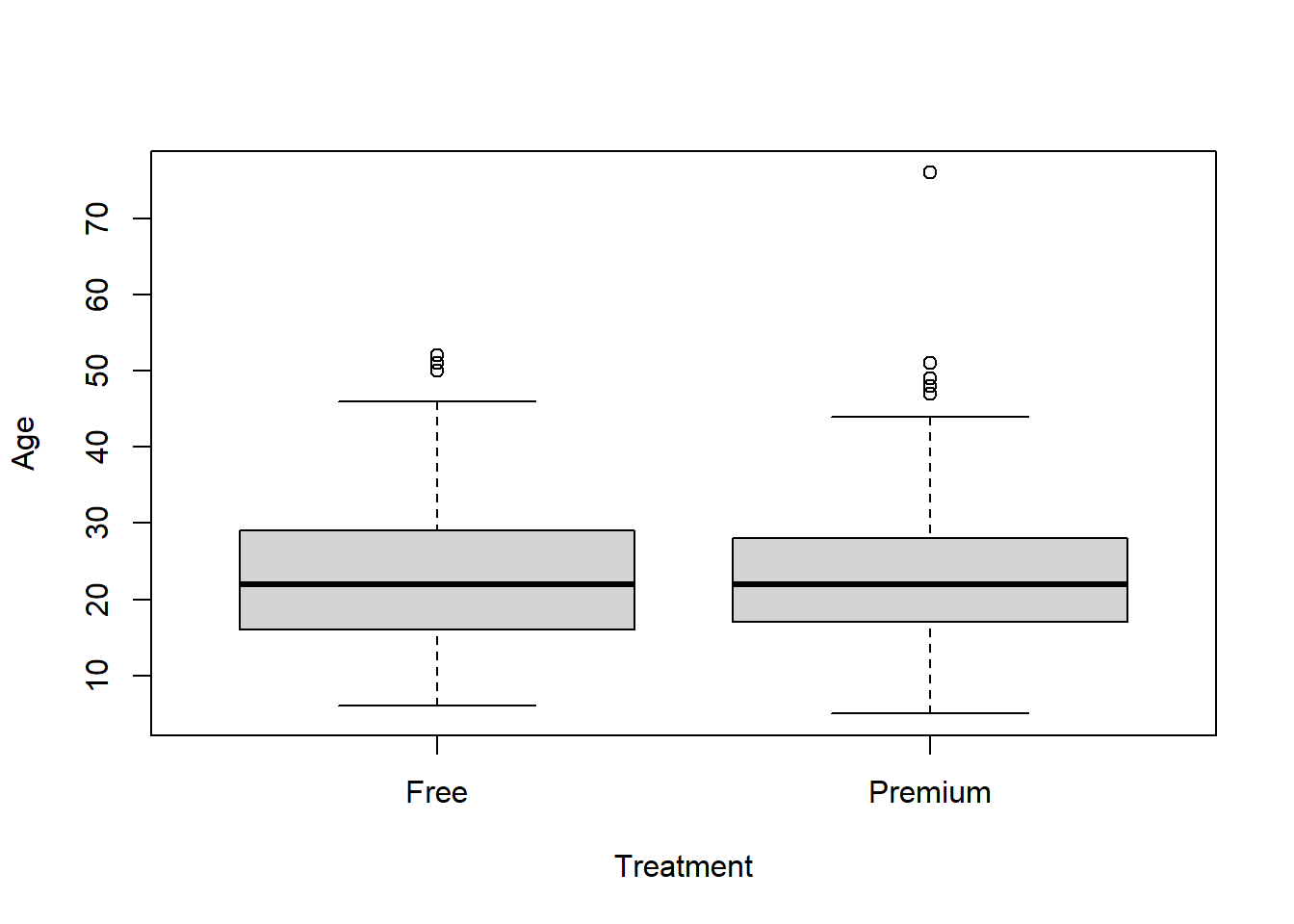
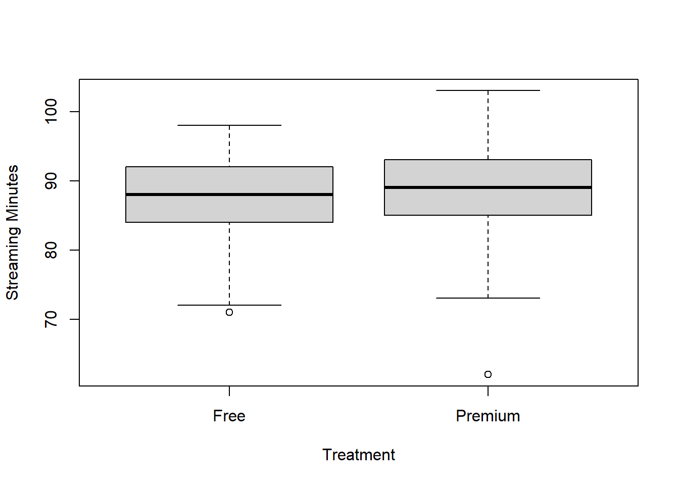
boxplot(musicfiExp$Age ~ musicfiExp$AccountType, ylab = "Age", xlab = "Treatment")

Age is not a confounding variable as it is independent of the treatment assignment. We can now directly attribute any differences in the outcome due to the intervention. This allows us to conclude that giving people a premium account increases streaming minutes.

boxplot(StreamingMinutes ~ AccountType, ylab = "Streaming Minutes", xlab = "Treatment")

t.test(musicfiExp$StreamingMinutes ~ musicfiExp$AccountType)

## 
##  Welch Two Sample t-test
## 
## data:  musicfiExp$StreamingMinutes by musicfiExp$AccountType
## t = -2.5057, df = 497.95, p-value = 0.01254
## alternative hypothesis: true difference in means is not equal to 0
## 95 percent confidence interval:
##  -2.2728058 -0.2750465
## sample estimates:
##    mean in group Free mean in group Premium 
##              87.55285              88.82677

The difference may be relatively small, but the low p-value indicates that the difference is statistically significant.

7.2.1 Designing an Experiment

Now that we know why experimentation is necessary, let’s review the steps that businesses use to design their experiments.

Generate a Hypothesis

The starting point to any experiment is to generate a hypothesis. For companies these hypotheses take the following form:

If we [do this] then [this outcome] will increase/decrease by [this much].

[do this]: describes the treatment; most of the time, we implicitly assume that the control is the current approach, and hence it is not explicitly mentioned.
[this outcome]: describes the outcome we expect the treatment will affect.
[this much]: describes our best guess at the likely effect of the treatment on the outcome. It is also essential to make a reasonable guess at what the effect will be; this guess will form the basis of a calculation that will determine the number of people (sample size) necessary to detect an effect of such a magnitude in an experiment.

Some examples:

If we enlarge our “Buy now” button by 20% then total sales will increase by +5%.
If we launch a simpler user interface on our home page then total sessions will increase by 10%.
If we remove fake accounts then complaints will decrease by 2%.

Although the above examples focus on a single outcome, it is common to look at one to five primary outcomes and possibly another ten to fifteen secondary (less important) outcomes. No matter the number, however, it is crucial that these are specified before data collection.

Select the Study Population

After generating the hypothesis, we have to identify the group(s) of people who will take part in the study; this is often called determining the inclusion/exclusion criteria. Choosing these criteria depends on the context.

For the above examples we could consider the following populations:

All U.S. cell phone users that visit the website.
All customers using the company’s iOS mobile application with version XXX or above.
All worldwide customers.

This step will provide us with an estimate of the overall population size. From here, we need to determine how we are going to recruit people into our study. The next step explains how to assign people to either treatment or control.

Define the Assignment Mechanism

The assignment mechanism is a probability distribution that specifies the likelihood of each person in our study receiving a treatment. There are, of course, many possible assignment mechanisms for an experiment on a population. Below, we introduce the two most popular mechanisms:

Bernoulli Design: Each person is independently assigned with probability \(p\) to receive the treatment and a probability \(1-p\) to receive the control. In other words, for every person, we toss an independent coin with probability of heads = \(p\), if we get heads, we assign them to treatment, and if we get tails, we assign them to control. This can be implemented using the sample() command with replace = TRUE.
Completely Randomized Design: In this design, we specify how many people will be placed in each condition. For example, we might specify that \(n_0\) will get the control and \(n_1\) will get the treatment. Then, we randomly pick \(n_0\) of our participants to receive the control and \(n_1\) to receive the treatment. This again can be implemented using the sample() command.

The main difference between a Bernoulli and a completely randomized design is that we guarantee how many people receive the treatment in the latter. On the other hand, the Bernoulli is much easier to implement if we don’t know exactly how many people will be in our study (e.g., people “arrive” one after another).

7.3 Power Analysis

After completing the steps in the previous section, businesses face an additional decision: how much data to collect in their experiment. Of course, more data is always better, but there are usually economic limitations that prevent one from collecting an arbitrarily large sample. Therefore, we face a trade-off: large samples may be prohibitively expensive, but if our sample is too small we may not have enough “power” to detect a significant difference between our treatment and control groups. That is, we may not have enough data to reject the null when there truly is a difference between the two groups. Power analysis allows us to calculate the minimum sample size required to detect a difference, given that one really exists.

Using the language of hypothesis testing from Section 5.3, Musicfi plans to test the following hypotheses, where \(\mu_0\) is the mean of the control group and \(\mu_1\) is the mean of the treatment group:

\(H_o: \mu_0 = \mu_1\)
\(H_a: \mu_0 \ne \mu_1\)

Imagine that the alternative hypothesis (\(H_a\)) is true, i.e., the mean streaming minutes is different for customers in the control and treatment groups. Even under this scenario, there is no guarantee that our analysis will detect the difference because we have a sample of customers (fortunately a random sample) and not the population of all possible customers. The question then becomes: what is the smallest sample we can collect that will still provide a reasonable chance of detecting a difference if one exists?

To tackle this question, think through the following scenarios. What do you think would require more data:

Detecting a difference in streaming time between free and premium users when the true average difference is five minutes, or
Detecting a difference when the true average difference is only two minutes?

Intuitively, the larger the true difference, the more likely that difference will manifest itself in our random sample. Therefore, we need would need more data in scenario (b) to pick up on the difference than we would in scenario (a).

Let’s imagine that based on the business context, Musicfi does not care if the difference between free and premium users is less than two minutes; in other words, if the true difference is two minutes or less, Musicfi would consider that difference negligible. Therefore, they want to determine the smallest possible sample size that still has a good chance of detecting a difference of two minutes or greater. Note this implies that if the true difference is less than two minutes, the experiment will likely not pick up on that difference. Determining the minimum detectable difference is an important step in a power analysis, and one that requires input from managers who have business area expertise.

To conduct a power analysis, we need several pieces of information:

The significance level of the test (\(\alpha\)). As before, we will use a significance level of 0.05.
The power of the test (\(1-\beta\)). This is the probability that our test will detect the difference given that there is a difference in the population. A common choice for \(1-\beta\) is 0.8. Note that this implies there is still a \(\beta\) = 20% chance our test will not detect the difference when a difference actually exists.
The treatment effect, defined as the difference between the two groups (\(\mu_1 - \mu_o\)). Of course, we don’t know the true population treatment effect — this is the quantity we are trying to estimate from the experiment. However, to determine how big our sample size should be, we need a plausible guess of the smallest effect that we would want to detect in our study. Typically, the estimate is based on historical data; we usually shrink the estimate closer to zero because our data is likely subject to unobserved confounding.
The pooled standard deviation of the two groups, usually estimated from historical data.

We then combine 3 and 4 to compute the normalized difference in means \(d\) (know as the effect size, or Cohen’s \(d\)) by dividing our estimate of the treatment effect by the pooled standard deviation.

For example, with the Musicfi data we want to observe a minimum difference of two minutes, so we would calculate \(d\) as:

\[d = \frac{\mu_1 - \mu_0}{s} = \frac{2}{s}\]

The quantity \(s\) is the pooled standard deviation of the two groups, and is calculated from the standard deviations of the control group and the treatment group (\(s_o\) and \(s_1\) respectively) using the formula below. These quantities typically need to be estimated from historical data; in our case, we can use the data from Musicfi’s previous experiment, which is stored in musicfiExp.

\[s = \sqrt{\frac{s_1^2 + s_0^2}{2}}\]

After determining the three inputs using our historical data, we use the pwr.t.test() function from R’s pwr package to calculate the required sample size.

pwr::pwr.t.test(d, power, sig.level=0.05)

Required arguments
- d: The effect size, i.e., Cohen’s \(d\).
- power: The power of the test (\(1-\beta\)).
Optional arguments
- conf.level: The significance level of the test.

Let’s say we want to design a new experiment that will have an 80% chance of detecting a difference of two minutes or greater at a 5% significance level. We can use the pwr.t.test() function to calculate the minimum sample size we will need for this experiment.

First, we need to calculate \(s\) based on our historical data:

# Create separate data frames for free and premium users
musicfiExpFree = subset(musicfiExp, AccountType=="Free")
musicfiExpPremium = subset(musicfiExp, AccountType=="Premium")

# Calculate the sample standard deviation of streaming minutes for free and premium users
s0 = sd(musicfiExpFree$StreamingMinutes)
s1 = sd(musicfiExpPremium$StreamingMinutes)

# Calculate the estimate of the pooled standard deviation
s = sqrt((s0^2 + s1^2)/2)

Now we can use s to calculate Cohen’s \(d\):

d = 2/s

Finally, we can apply the pwr.t.test() function to determine our sample size:

pwr.t.test(d=d, power=0.8)

## 
##      Two-sample t test power calculation 
## 
##               n = 127.7748
##               d = 0.3518408
##       sig.level = 0.05
##           power = 0.8
##     alternative = two.sided
## 
## NOTE: n is number in *each* group

These results indicate that (rounding up) we need at least 128 participants in the control and treatment groups, for a total sample size of 256.