Chapter 3 Wrangling Data
Unfortunately, data does not often come presented on a silver platter. It may contain mistakes, such as data entry errors, or simply not be in a format that is conducive to easy analysis. Therefore, the first step in any data analysis task is typically cleaning, organizing, and re-formatting the data, which is collectively referred to as data wrangling. These topics are covered in this chapter.
3.1 A Brief Note on Packages
As we noted in Section 1.2.1, we will be relying on a set of packages known as the tidyverse to help process data in R. In general, there are two steps you must complete to use a package in R:
Install the package - To use a package in R, that package must be installed on the machine where you are running your code. Typically, you can install packages using the following code:
install.packages(“packageName”)
Load the package - Once the package is installed, you need to load it into your R session using the following code:
library(packageName)
Because we are using the tidyverse, we need to install and load thetidyversepackage:
The output provides us with some information on the installation process, and can be ignored.
Note that in the install.packages() function, tidyverse needs to be in quotation marks, but in the library() function it should not be in quotation marks.
Once a package is installed on a machine, it does not need to be re-installed in the future. This means that if you run your code on the same computer all the time, you will only need to run the install.packages() function once (the first time you use the package). Then, each subsequent time you use the package, it will already be installed and you can simply load it with the library() function.
Note: Finally, just a word of caution - the code we will use in this chapter relies on the tidyverse, which means that much of it will not work if you fail to load the tidyverse package at the start of your R session.
3.2 Reading in Data
The tidyverse contains a variety of functions for reading in data from different file types. Our employee data is saved in a comma-separated values (.csv) file called employee_data.csv. We can read the data from this file into a data frame using the read_csv() function, which uses the following syntax:
tidyverse::read_csv(file, col_names=TRUE, skip=0, …)
- Required arguments
file: The file path of the file you would like to read in. Note that the path must be surrounded in quotation marks.
- Optional arguments
col_names: When this argument isTRUE, the first row of the file is assumed to contain the column names of the data set. When it isFALSE, the first row is assumed to contain data, and column names are generated automatically (X1,X2,X3, etc.)skip: The number of rows at the top of the file to skip when reading in the data. This is useful if the first few rows of your data file have text you want to ignore.
Below we use this function to read our data from the csv file into a data frame called employees.
## Rows: 1000 Columns: 10## -- Column specification --------------------------------------------------------
## Delimiter: ","
## chr (6): Name, Gender, Degree, Start_Date, Division, Salary
## dbl (3): ID, Age, Rating
## lgl (1): Retired##
## i Use `spec()` to retrieve the full column specification for this data.
## i Specify the column types or set `show_col_types = FALSE` to quiet this message.By default, the function prints out the assumed data type of each column. For example, the function assumes that ID is a double (a sub-class of the numeric type), Name is a character, Retired is a logical, etc. These seem like the correct choices. However, you may also notice that the function got some of the types wrong. For example, Start_Date, Degree, and Salary were all read in as characters instead of as a Date, factor, and numeric, respectively. We will see how to correct this in section 3.4.
If our data were in an Excel (.xlsx) file instead of a csv, we could read it in using the read_excel() function from the readxl package (Wickham and Bryan 2019). This function uses the following syntax:
readxl::read_excel(file, sheet=1, col_names=TRUE, range=NULL, skip=0 …)
- Required arguments
file: The file path of the file you would like to read in. Note that the path must be surrounded in quotation marks.
- Optional arguments
sheet: The sheet within the Excel workbook that contains the data you want to read in. You can either specify the sheet number (the default issheet=1), or the name of the sheet as a string (e.g.,sheet="Sheet Name").col_names: When this argument isTRUE, the first row of the file is assumed to contain the column names of the data set. When it isFALSE, the first row is assumed to contain data, and column names are generated automatically (X1,X2,X3, etc.)range: The range of cells in the sheet that contains the data you would like to read in. For example, if your only wanted to read in the data in the rangeB4:F100, you would setrange="B4:F100".skip: The number of rows at the top of the file to skip when reading in the data. This is useful if the first few rows of your data file have text you want to ignore.
Although .csv and .xlsx are very common file types, you will likely encounter data stored in other file types (tab-separated files (.tab), text files (.txt), etc.) Here we will not show the functions to read in data from all of these different file types. However, they will generally be of a similar form as the read_csv() and read_excel() functions shown above. Always start by Googling to find the appropriate function for the type of file you need to read into R.
3.3 Data Frame Basics
Now that our employee data has been read into a data frame, we can begin exploring the data! We will start by exploring the dimensions of the data set. We can determine the number of rows (or observations) in our data set with the nrow() function:
nrow(df)
## [1] 1000Similarly, we can use ncol() to determine the number of columns:
ncol(df)
## [1] 10The dim() function returns the full dimensions of the data (i.e., both the number of rows and columns):
dim(df)
## [1] 1000 10We can view the first and last few rows of the data set with the head() and tail() functions, respectively:
head(df) & tail(df)
## # A tibble: 6 x 10
##      ID Name     Gender   Age Rating Degree   Start_Date Retired Division Salary
##   <dbl> <chr>    <chr>  <dbl>  <dbl> <chr>    <chr>      <lgl>   <chr>    <chr>
## 1  6881 al-Rahi~ Female    51     10 High Sc~ 2/23/90    FALSE   Operati~ $108,~
## 2  2671 Lewis, ~ Male      34      4 Ph.D     2/23/07    FALSE   Enginee~ $182,~
## 3  8925 el-Jaff~ Female    50     10 Master's 2/23/91    FALSE   Enginee~ $206,~
## 4  2769 Soto, M~ Male      52     10 High Sc~ 2/23/87    FALSE   Sales    $183,~
## 5  2658 al-Ebra~ Male      55      8 Ph.D     2/23/85    FALSE   Corpora~ $236,~
## 6 1933 Medina,~ Female 62 7 Associa~ 2/23/79 TRUE Sales <NA>## # A tibble: 6 x 10
## ID Name Gender Age Rating Degree Start_Date Retired Division Salary
## <dbl> <chr> <chr> <dbl> <dbl> <chr> <chr> <lgl> <chr> <chr>
## 1 6681 Bruns, ~ Male 41 8 Ph.D 2/23/02 FALSE Engineer~ $188,~
## 2 2031 Martine~ Male 57 8 Ph.D 2/23/84 FALSE Engineer~ $218,~
## 3 2066 Gonzale~ Female 32 2 High S~ 2/23/08 FALSE Operatio~ $84,0~
## 4 3239 Larson,~ Male 37 5 Bachel~ 2/23/02 FALSE Human Re~ $149,~
## 5 3717 Levy-Mi~ Male 53 10 Bachel~ 2/23/89 FALSE Operatio~ $172,~
## 6 4209 Dena, G~ Female 49 6 Master~ 2/23/91 FALSE Accounti~ $185,~It is easy to get a quick view of the structure of the data using the str() function. This shows the number of observations, the number of variables, the type of each variable, and the first few values of each variable.
str(df)
## spec_tbl_df [1,000 x 10] (S3: spec_tbl_df/tbl_df/tbl/data.frame)
##  $ ID        : num [1:1000] 6881 2671 8925 2769 2658 ...
##  $ Name      : chr [1:1000] "al-Rahimi, Tayyiba" "Lewis, Austin" "el-Jaffer, Manaal" "Soto, Michael" ...
##  $ Gender    : chr [1:1000] "Female" "Male" "Female" "Male" ...
##  $ Age       : num [1:1000] 51 34 50 52 55 62 47 43 27 30 ...
##  $ Rating    : num [1:1000] 10 4 10 10 8 7 8 8 7 6 ...
##  $ Degree    : chr [1:1000] "High School" "Ph.D" "Master's" "High School" ...
##  $ Start_Date: chr [1:1000] "2/23/90" "2/23/07" "2/23/91" "2/23/87" ...
##  $ Retired   : logi [1:1000] FALSE FALSE FALSE FALSE FALSE TRUE ...
##  $ Division  : chr [1:1000] "Operations" "Engineering" "Engineering" "Sales" ...
##  $ Salary    : chr [1:1000] "$108,804" "$182,343" "$206,770" "$183,407" ...
##  - attr(*, "spec")=
##   .. cols(
##   ..   ID = col_double(),
##   ..   Name = col_character(),
##   ..   Gender = col_character(),
##   ..   Age = col_double(),
##   ..   Rating = col_double(),
##   ..   Degree = col_character(),
##   ..   Start_Date = col_character(),
##   ..   Retired = col_logical(),
##   ..   Division = col_character(),
##   ..   Salary = col_character()
##   .. )
##  - attr(*, "problems")=<externalptr>
After reading in a data set, it is best practice to start by checking the dimensions of the data and exploring its structure using the functions shown in this section. This will help uncover any immediate problems with the data.
So far we have seen some functions that can applied to an entire data frame. However, we often want to work with an individual column in a data frame. For example, we may be interested in calculating the average Age of all employees in the data set. We can access specific columns of a data frame using the $ operator, which takes the general form:
df$varName
If we write employees$Age, we will get an atomic vector with the age of the 1,000 employees in the data frame. If you recall from Section 2.3.1, there are many different functions we can apply to atomic vectors in R. Because employees$Age is an atomic vector, we can apply those functions here to explore the Age variable. For example, to calculate the mean, minimum, and maximum Age, we could write:
## [1] 45.53## [1] 25## [1] 653.4 Fixing Variable Types
As we saw when we read in the data in Section 3.2, R does not always correctly guess the appropriate type for our columns. This is a very common occurance, and fixing column types is a tedious but important step in preparing a data frame for analysis.
3.4.1 Fixing Numeric Variables
When the read_csv() function read in the data, it assumed that the Salary column was a character instead of a numeric. This is because the data includes dollar signs ($), commas (,), and periods (.), which R interprets as characters. Fortunately, it is very easy to correct this using the parse_number() function from the tidyverse, which uses the following syntax:
tidyverse::parse_number(x, locale = default_locale(), …)
- Required arguments
x: An atomic vector with values you would like to convert to anumeric.
- Optional arguments
locale: This is used to control the parsing convention for numbers. By default, the function assumes that periods (.) are used for decimal marks and commas (,) are used for grouping (e.g., numbers are written as $1,500.25). You can explicitly change the characters that are used for decimal marks and groupings by setting changing thegrouping_markanddecimal_mark, respectively. For example, if numbers are written in the European convention (e.g., numbers are written as €1.500,25), you could setlocale=locale(grouping_mark=".", decimal_mark=",").
Let’s first trying applying this function to a single value to see how it works:
## [1] 1500.25If our data is recorded in a different format, we can explicitly set the decimal mark and grouping characters in the locale argument so that the data is converted properly:
## [1] 1500.25To convert the entire Salary column to a numeric, we can apply parse_number() to the entire column, and then store the parsed values back into the Salary column:
Now if we view the class of Salary, it will show numeric:
## [1] "numeric"Finally, if we view the first few rows of our data frame with head(), we’ll see that Salary no longer contains dollar signs, decimals, or commas:
## # A tibble: 6 x 10
##      ID Name      Gender   Age Rating Degree  Start_Date Retired Division Salary
##   <dbl> <chr>     <chr>  <dbl>  <dbl> <chr>   <chr>      <lgl>   <chr>     <dbl>
## 1  6881 al-Rahim~ Female    51     10 High S~ 2/23/90    FALSE   Operati~ 108804
## 2  2671 Lewis, A~ Male      34      4 Ph.D    2/23/07    FALSE   Enginee~ 182343
## 3  8925 el-Jaffe~ Female    50     10 Master~ 2/23/91    FALSE   Enginee~ 206770
## 4  2769 Soto, Mi~ Male      52     10 High S~ 2/23/87    FALSE   Sales    183407
## 5  2658 al-Ebrah~ Male      55      8 Ph.D    2/23/85    FALSE   Corpora~ 236240
## 6  1933 Medina, ~ Female    62      7 Associ~ 2/23/79    TRUE    Sales        NA
3.4.2 Fixing Factor Variables
Similarly, we can use tidyverse’s parse_factor() function to convert the Degree column to a factor. This function uses the following syntax:
tidyverse::parse_factor(x, levels=NULL, ordered=FALSE, …)
- Required arguments
x: An atomic vector with values you would like to convert to afactor.
- Optional arguments
levels: An atomic vector with the unique values of the factor. If the default ofNULLis used, the function automatically determines the levels based on the data.ordered: Used to determine whether the factor levels are ordered or not. For example, if we had a factor that was coded as “small”, “medium”, and “large”, we would setordered=TRUEbecause there is an ordering to these levels.
In the code below, we first create an atomic vector called degreeLevels with the values of our factor. Then, we use parse_factor() to convert the Degree column from a character to a factor. Note that we set ordered=TRUE to acknowledge that there is an ordering to the five degrees.
degreeLevels <- c("High School", "Associate's", "Bachelor's", "Master's", "Ph.D")
employees$Degree <- parse_factor(employees$Degree, levels = degreeLevels, ordered = TRUE)
Now if we view the class of Degree, it will show factor:
## [1] "ordered" "factor"3.4.3 Fixing Date Variables
As you might expect, the tidyverse also has a parse_date() function that we can use to convert the Start_Date column to a Date. This function uses the following syntax:
tidyverse::parse_date(x, format="", …)
- Required arguments
x: An atomic vector with values you would like to convert to aDate.
- Optional arguments
format: The format of the date. Because dates can be recorded in a variety of ways, R has a set of symbols that can be used to represent different date formats:
| Symbol | Meaning | Example |
|---|---|---|
| %d | day as a number | 01-31 |
| %a | abbreviated weekday | Mon |
| %A | unabbreviated weekday | Monday |
| %m | month (00-12) | 00-12 |
| %b | abbreviated month | Jan |
| %B | unabbreviated month | January |
| %y | 2-digit year | 07 |
| %Y | 4-digit year | 2007 |
Source: here.
Below we see some examples of the parse_date() function applied to dates of different formats:
## [1] "1999-06-25"## [1] "2021-01-12"## [1] "1995-08-18"## [1] "2003-02-12"Now we’ll use the format_date() function to convert the entire Start_Date column to a Date. This column is coded as month/day/year, so the format of our date is %m/%d/%Y.
Now if we view the class of Start_Date, it will show Date:
## [1] "Date"3.5 Manipulating Data
3.5.1 Sorting Data
Often you would like to sort your data based on one or more of the columns in your data set. This can be done using the arrange() function, which uses the following syntax:
tidyverse::arrange(df, var1, var2, var3, …)
- Required arguments
df: The tibble (data frame) with the data you would like to sort.var1: The name of the column to use to sort the data.
- Optional arguments
var2, var3, ...: The name of additional columns to use to sort the data. When multiple columns are specified, each additional column is used to break ties in the preceding column.
By default, arrange() sorts numeric variables from smallest to largest and character variables alphabetically. You can reverse the order of the sort by surrounding the column name with desc() in the function call.
First, let’s create a new version of the data frame called employeesSortedAge, with the employees sorted from youngest to oldest.
## # A tibble: 6 x 10
##      ID Name     Gender   Age Rating Degree  Start_Date Retired Division  Salary
##   <dbl> <chr>    <chr>  <dbl>  <dbl> <ord>   <date>     <lgl>   <chr>      <dbl>
## 1  7068 Dimas, ~ Male      25      8 High S~ 2017-02-23 FALSE   Operatio~  84252
## 2  5464 al-Pira~ Male      25      3 Associ~ 2016-02-23 FALSE   Operatio~  37907
## 3  7910 Hopper,~ Female    25      7 Bachel~ 2017-02-23 FALSE   Engineer~ 100688
## 4  6784 al-Sidd~ Female    25      4 Master~ 2015-02-23 FALSE   Human Re~ 127618
## 5  3240 Steggal~ Female    25      7 Master~ 2017-02-23 FALSE   Operatio~ 117062
## 6 1413 Tanner,~ Male 25 2 Associ~ 2016-02-23 FALSE Operatio~ 61869## # A tibble: 6 x 10
## ID Name Gender Age Rating Degree Start_Date Retired Division Salary
## <dbl> <chr> <chr> <dbl> <dbl> <ord> <date> <lgl> <chr> <dbl>
## 1 6798 Werkele~ Male 65 7 Ph.D 1976-02-23 TRUE Enginee~ NA
## 2 6291 Anderso~ Male 65 6 High Sc~ 1977-02-23 FALSE Operati~ 179634
## 3 8481 Phillip~ Female 65 5 High Sc~ 1975-02-23 TRUE Sales NA
## 4 4600 Olivas,~ Male 65 2 Ph.D 1976-02-23 FALSE Enginee~ 204576
## 5 6777 Mortime~ Female 65 7 Master's 1977-02-23 FALSE Corpora~ 248925
## 6 2924 Mills, ~ Female 65 8 High Sc~ 1977-02-23 FALSE Operati~ 138212We can instead sort the data from oldest to youngest by adding desc() around Age:
## # A tibble: 6 x 10
##      ID Name     Gender   Age Rating Degree  Start_Date Retired Division  Salary
##   <dbl> <chr>    <chr>  <dbl>  <dbl> <ord>   <date>     <lgl>   <chr>      <dbl>
## 1  8060 al-Mora~ Male      65      8 Ph.D    1977-02-23 FALSE   Corporate 213381
## 2  9545 Lloyd, ~ Male      65      9 Bachel~ 1974-02-23 FALSE   Accounti~ 243326
## 3  7305 Law, Ch~ Female    65      8 Associ~ 1976-02-23 FALSE   Human Re~ 214788
## 4  4141 Herrera~ Female    65      8 High S~ 1975-02-23 FALSE   Operatio~ 143728
## 5  2559 Holiday~ Female    65      7 Bachel~ 1975-02-23 TRUE    Operatio~     NA
## 6 4407 Ross, C~ Female 65 7 Bachel~ 1975-02-23 TRUE Corporate NA## # A tibble: 6 x 10
## ID Name Gender Age Rating Degree Start_Date Retired Division Salary
## <dbl> <chr> <chr> <dbl> <dbl> <ord> <date> <lgl> <chr> <dbl>
## 1 1413 Tanner,~ Male 25 2 Associa~ 2016-02-23 FALSE Operati~ 61869
## 2 8324 Bancrof~ Male 25 7 Master's 2017-02-23 FALSE Corpora~ 135935
## 3 1230 Kirgis,~ Female 25 8 Bachelo~ 2015-02-23 FALSE Operati~ 113573
## 4 6308 Barnett~ Male 25 8 Master's 2016-02-23 FALSE Operati~ 103798
## 5 3241 Byrd, S~ Female 25 6 Ph.D 2016-02-23 FALSE Enginee~ 126366
## 6 9249 Lopez, ~ Female 25 8 Associa~ 2016-02-23 FALSE Sales 75689Now imagine that we wanted to perform a multi-level sort, where we first sort the employees from oldest to youngest, and then within each age sort the names alphabetically. We can do this by adding the Name column to our function call:
## # A tibble: 6 x 10
##      ID Name     Gender   Age Rating Degree   Start_Date Retired Division Salary
##   <dbl> <chr>    <chr>  <dbl>  <dbl> <ord>    <date>     <lgl>   <chr>     <dbl>
## 1  8060 al-Mora~ Male      65      8 Ph.D     1977-02-23 FALSE   Corpora~ 213381
## 2  6291 Anderso~ Male      65      6 High Sc~ 1977-02-23 FALSE   Operati~ 179634
## 3  3661 el-Mesk~ Male      65      9 Bachelo~ 1977-02-23 FALSE   Enginee~ 177504
## 4  5245 Gowen, ~ Female    65      7 Bachelo~ 1975-02-23 FALSE   Account~ 191765
## 5  4141 Herrera~ Female    65      8 High Sc~ 1975-02-23 FALSE   Operati~ 143728
## 6 2559 Holiday~ Female 65 7 Bachelo~ 1975-02-23 TRUE Operati~ NA## # A tibble: 6 x 10
## ID Name Gender Age Rating Degree Start_Date Retired Division Salary
## <dbl> <chr> <chr> <dbl> <dbl> <ord> <date> <lgl> <chr> <dbl>
## 1 7068 Dimas, ~ Male 25 8 High Sc~ 2017-02-23 FALSE Operati~ 84252
## 2 7910 Hopper,~ Female 25 7 Bachelo~ 2017-02-23 FALSE Enginee~ 100688
## 3 1230 Kirgis,~ Female 25 8 Bachelo~ 2015-02-23 FALSE Operati~ 113573
## 4 9249 Lopez, ~ Female 25 8 Associa~ 2016-02-23 FALSE Sales 75689
## 5 3240 Steggal~ Female 25 7 Master's 2017-02-23 FALSE Operati~ 117062
## 6 1413 Tanner,~ Male 25 2 Associa~ 2016-02-23 FALSE Operati~ 618693.5.2 Filtering Rows
Instead of just sorting the rows in your data, you might want to filter out rows based on a set of conditions. You can do this with the filter() function, which uses the following syntax:
tidyverse::filter(df, condition1, condition2, condition3, …)
- Required arguments
df: The tibble (data frame) with the data you would like to filter.condition1: The logical condition that identifies the rows you would like to keep.
- Optional arguments
condition2, condition3, ...: Any additional conditions that identify the rows you would like to keep.
The conditions specified in filter() can use a variety of comparison operators:
>(greater than),<(less than)>=(greater than or equal to),<=(less than or equal to)==(equal to); note that a single equals sign (=) will not work!=(not equal to)
For example, imagine we wanted to create a new data frame with only those employees who are retired. We could do this with filter() by writing a condition that specifies that the Retired variable equals TRUE:
## # A tibble: 6 x 10
##      ID Name      Gender   Age Rating Degree  Start_Date Retired Division Salary
##   <dbl> <chr>     <chr>  <dbl>  <dbl> <ord>   <date>     <lgl>   <chr>     <dbl>
## 1  1933 Medina, ~ Female    62      7 Associ~ 1979-02-23 TRUE    Sales        NA
## 2  9259 Armantro~ Female    61      7 Associ~ 1980-02-23 TRUE    Operati~     NA
## 3  6223 Ali, Mic~ Female    60      7 Ph.D    1982-02-23 TRUE    Corpora~     NA
## 4  5955 al-Youne~ Male      63      7 High S~ 1979-02-23 TRUE    Sales        NA
## 5  6195 Tolbert,~ Female    60      8 High S~ 1983-02-23 TRUE    Sales        NA
## 6 9620 Medina, ~ Male 61 2 Master~ 1980-02-23 TRUE Account~ NA## [1] 80 10By specifying multiple conditions in our call to filter(), we can filter by more than one rule. Let’s say we wanted a dataset with employees who:
- Are still working, and
- Started on or after January 1, 1995, and
- Are not in human resources.
employeesSub <- filter(employees,
                       Retired == FALSE, Start_Date >= "1995-01-01", Division != "Operations")
head(employeesSub)
## # A tibble: 6 x 10
## ID Name Gender Age Rating Degree Start_Date Retired Division Salary
## <dbl> <chr> <chr> <dbl> <dbl> <ord> <date> <lgl> <chr> <dbl>
## 1 2671 Lewis, ~ Male 34 4 Ph.D 2007-02-23 FALSE Engineer~ 182343
## 2 7821 Hollema~ Female 43 8 Master~ 1999-02-23 FALSE Human Re~ 149468
## 3 5915 Rogers,~ Female 27 2 Bachel~ 2013-02-23 FALSE Human Re~ 79183
## 4 9871 Sontag,~ Female 30 7 Ph.D 2011-02-23 FALSE Engineer~ 164384
## 5 2828 el-Ulla~ Female 42 5 Bachel~ 1999-02-23 FALSE Sales 138973
## 6 2836 Ochoa, ~ Male 41 7 Bachel~ 1999-02-23 FALSE Corporate 152011## [1] 376 10When you list multiple conditions in filter(), those conditions are combined with “and”. In the previous example, our new data frame employeesSub contains the 376 employees who are still working, and who started on or after January 1, 1995, and who are not in human resources.
However, you might want to filter based on one condition or another. For example, imagine we wanted to find all employees who have a master’s, or who started on or before December 31, 2000, or who make less than $100,000. To do this, instead of listing each condition as a separate argument, we combine the conditions with the | character, which evaluates to “or”. For example:
employeesSubOr <- filter(employees,
                         Degree == "Master's" | Start_Date <= "2000-12-31" | Salary < 100000)
head(employeesSubOr)
## # A tibble: 6 x 10
## ID Name Gender Age Rating Degree Start_Date Retired Division Salary
## <dbl> <chr> <chr> <dbl> <dbl> <ord> <date> <lgl> <chr> <dbl>
## 1 6881 al-Rahim~ Female 51 10 High S~ 1990-02-23 FALSE Operati~ 108804
## 2 8925 el-Jaffe~ Female 50 10 Master~ 1991-02-23 FALSE Enginee~ 206770
## 3 2769 Soto, Mi~ Male 52 10 High S~ 1987-02-23 FALSE Sales 183407
## 4 2658 al-Ebrah~ Male 55 8 Ph.D 1985-02-23 FALSE Corpora~ 236240
## 5 1933 Medina, ~ Female 62 7 Associ~ 1979-02-23 TRUE Sales NA
## 6 3570 Troftgru~ Female 47 8 High S~ 1995-02-23 FALSE Operati~ 101138## [1] 741 10Now let’s create a data frame with the employees who have a Master’s or a Ph.D. We could do this using the or operator |:
## # A tibble: 6 x 10
##      ID Name      Gender   Age Rating Degree Start_Date Retired Division  Salary
##   <dbl> <chr>     <chr>  <dbl>  <dbl> <ord>  <date>     <lgl>   <chr>      <dbl>
## 1  2671 Lewis, A~ Male      34      4 Ph.D   2007-02-23 FALSE   Engineer~ 182343
## 2  8925 el-Jaffe~ Female    50     10 Maste~ 1991-02-23 FALSE   Engineer~ 206770
## 3  2658 al-Ebrah~ Male      55      8 Ph.D   1985-02-23 FALSE   Corporate 236240
## 4  7821 Holleman~ Female    43      8 Maste~ 1999-02-23 FALSE   Human Re~ 149468
## 5  9871 Sontag, ~ Female    30      7 Ph.D   2011-02-23 FALSE   Engineer~ 164384
## 6 2687 Benavide~ Male 45 8 Ph.D 1997-02-23 FALSE Engineer~ 181924## [1] 400 10Now imagine we wanted to find all employees who have a Master’s, a Ph.D, or a Bachelor’s. We could add another | to our condition and specify that Degree == "Bachelor's". Alternatively, we could make our code more compact by re-writing the condition as var_name %in% values. This will filter to only those rows where var_name is equal to one of the values specified in the atomic vector values. For example:
employeesCollege <- filter(employees, Degree %in% c("Bachelor's", "Master's", "Ph.D"))
head(employeesCollege)
## # A tibble: 6 x 10
## ID Name Gender Age Rating Degree Start_Date Retired Division Salary
## <dbl> <chr> <chr> <dbl> <dbl> <ord> <date> <lgl> <chr> <dbl>
## 1 2671 Lewis, ~ Male 34 4 Ph.D 2007-02-23 FALSE Engineer~ 182343
## 2 8925 el-Jaff~ Female 50 10 Master~ 1991-02-23 FALSE Engineer~ 206770
## 3 2658 al-Ebra~ Male 55 8 Ph.D 1985-02-23 FALSE Corporate 236240
## 4 7821 Hollema~ Female 43 8 Master~ 1999-02-23 FALSE Human Re~ 149468
## 5 5915 Rogers,~ Female 27 2 Bachel~ 2013-02-23 FALSE Human Re~ 79183
## 6 9871 Sontag,~ Female 30 7 Ph.D 2011-02-23 FALSE Engineer~ 164384## [1] 600 10
Be careful filtering data when you have missing values (NA).
The filter() function keeps only those rows where the specified condition(s) evaluate(s) to TRUE. This is complicated by the presence of missing values, as it is impossible to determine whether a condition is TRUE or FALSE if the relevant information is missing. In our employees data set, we are missing a Salary for around 5% of the employees. If we wanted to filter to only those individuals who made more than $100,000, how would filter() treat the 5% of employees with NA values for Salary? Because the condition does not evaluate to TRUE for these rows, they are dropped.
## # A tibble: 6 x 10
##      ID Name      Gender   Age Rating Degree  Start_Date Retired Division Salary
##   <dbl> <chr>     <chr>  <dbl>  <dbl> <ord>   <date>     <lgl>   <chr>     <dbl>
## 1  6881 al-Rahim~ Female    51     10 High S~ 1990-02-23 FALSE   Operati~ 108804
## 2  2671 Lewis, A~ Male      34      4 Ph.D    2007-02-23 FALSE   Enginee~ 182343
## 3  8925 el-Jaffe~ Female    50     10 Master~ 1991-02-23 FALSE   Enginee~ 206770
## 4  2769 Soto, Mi~ Male      52     10 High S~ 1987-02-23 FALSE   Sales    183407
## 5  2658 al-Ebrah~ Male      55      8 Ph.D    1985-02-23 FALSE   Corpora~ 236240
## 6  3570 Troftgru~ Female    47      8 High S~ 1995-02-23 FALSE   Operati~ 101138
In this example, employees100k would not include any of the employees whose salary is unknown. Note that R provides no warning that these rows are being excluded as well; it is up to the user to recognize that the data contains missing values, and that this will affect how data are filtered.
If you did not want R to drop the missing values, you could explicitly state in the condition to keep all rows where Salary is greater than or equal to $100,000, or where Salary is missing. As we saw before, we can combine conditions with “or” using the | character. It may be tempting to assume we should add Salary == NA in order to capture the rows where Salary is missing; however, this will not work. We cannot use logical operators like == to compare something to NA. Instead have to use the is.na(), as follows:
## # A tibble: 6 x 10
##      ID Name      Gender   Age Rating Degree  Start_Date Retired Division Salary
##   <dbl> <chr>     <chr>  <dbl>  <dbl> <ord>   <date>     <lgl>   <chr>     <dbl>
## 1  6881 al-Rahim~ Female    51     10 High S~ 1990-02-23 FALSE   Operati~ 108804
## 2  2671 Lewis, A~ Male      34      4 Ph.D    2007-02-23 FALSE   Enginee~ 182343
## 3  8925 el-Jaffe~ Female    50     10 Master~ 1991-02-23 FALSE   Enginee~ 206770
## 4  2769 Soto, Mi~ Male      52     10 High S~ 1987-02-23 FALSE   Sales    183407
## 5  2658 al-Ebrah~ Male      55      8 Ph.D    1985-02-23 FALSE   Corpora~ 236240
## 6 1933 Medina, ~ Female 62 7 Associ~ 1979-02-23 TRUE Sales NA## # A tibble: 6 x 10
## ID Name Gender Age Rating Degree Start_Date Retired Division Salary
## <dbl> <chr> <chr> <dbl> <dbl> <ord> <date> <lgl> <chr> <dbl>
## 1 5271 Leschin~ Female 36 4 Ph.D 2004-02-23 FALSE Corporate 160364
## 2 6681 Bruns, ~ Male 41 8 Ph.D 2002-02-23 FALSE Engineer~ 188656
## 3 2031 Martine~ Male 57 8 Ph.D 1984-02-23 FALSE Engineer~ 218430
## 4 3239 Larson,~ Male 37 5 Bachel~ 2002-02-23 FALSE Human Re~ 149789
## 5 3717 Levy-Mi~ Male 53 10 Bachel~ 1989-02-23 FALSE Operatio~ 172703
## 6 4209 Dena, G~ Female 49 6 Master~ 1991-02-23 FALSE Accounti~ 185445Our new data frame, employees100kNA, contains all employees whose Salary is greater than $100,000, or whose Salary is missing from the data.
3.5.3 Selecting Columns
In the previous section we saw how to select certain rows based on a set of conditions. In this section we show how to select certain columns, which we can do with select():
tidyverse::select(df, var1, var2, var3, …)
- Required arguments
df: The tibble (data frame) with the data.var1: The name of the column to keep.
- Optional arguments
var2, var3, ...: The name of additional columns to keep.
Imagine we wanted to explore the relationship between Degree, Division, and Salary, and did not care about any of the other columns in the employees data set. Using select(), we could create a new data frame with only those columns:
## # A tibble: 6 x 3
##   Degree      Division    Salary
##   <ord>       <chr>        <dbl>
## 1 High School Operations  108804
## 2 Ph.D        Engineering 182343
## 3 Master's    Engineering 206770
## 4 High School Sales       183407
## 5 Ph.D        Corporate   236240
## 6 Associate's Sales           NA
If we want to exclude column(s) by name, we can simply add a minus sign in front of the column names in the call to filter():
## # A tibble: 6 x 8
##      ID Name                Gender Rating Degree      Start_Date Division Salary
##   <dbl> <chr>               <chr>   <dbl> <ord>       <date>     <chr>     <dbl>
## 1  6881 al-Rahimi, Tayyiba  Female     10 High School 1990-02-23 Operati~ 108804
## 2  2671 Lewis, Austin       Male        4 Ph.D        2007-02-23 Enginee~ 182343
## 3  8925 el-Jaffer, Manaal   Female     10 Master's    1991-02-23 Enginee~ 206770
## 4  2769 Soto, Michael       Male       10 High School 1987-02-23 Sales    183407
## 5  2658 al-Ebrahimi, Mamoon Male        8 Ph.D        1985-02-23 Corpora~ 236240
## 6  1933 Medina, Brandy      Female      7 Associate's 1979-02-23 Sales        NA
3.5.4 Creating New Columns
A very powerful function in the tidyverse is mutate(), which allows us to create new columns based on existing ones.
tidyverse::mutate(df, newVar1 = …, newVar2 = …, newVar3 = …, …)
- Required arguments
df: The tibble (data frame) with the data.newVar1 = ...: The new column to create.
- Optional arguments
newVar2 = ..., newVar3 = ..., ...: Any additional columns to create.
Let’s start with a simple example. Imagine we wanted to calculate the employees’ salaries in Euros instead of dollars. At the time of writing, the conversion rate was about €1 / $1.21, which means we need to divide everyone’s Salary in dollars by 1.21. Below we will use mutate() to create a new column called SalaryEu:
## # A tibble: 6 x 11
##      ID Name      Gender   Age Rating Degree  Start_Date Retired Division Salary
##   <dbl> <chr>     <chr>  <dbl>  <dbl> <ord>   <date>     <lgl>   <chr>     <dbl>
## 1  6881 al-Rahim~ Female    51     10 High S~ 1990-02-23 FALSE   Operati~ 108804
## 2  2671 Lewis, A~ Male      34      4 Ph.D    2007-02-23 FALSE   Enginee~ 182343
## 3  8925 el-Jaffe~ Female    50     10 Master~ 1991-02-23 FALSE   Enginee~ 206770
## 4  2769 Soto, Mi~ Male      52     10 High S~ 1987-02-23 FALSE   Sales    183407
## 5  2658 al-Ebrah~ Male      55      8 Ph.D    1985-02-23 FALSE   Corpora~ 236240
## 6  1933 Medina, ~ Female    62      7 Associ~ 1979-02-23 TRUE    Sales        NA
## # ... with 1 more variable: SalaryEu <dbl>
Note that mutate() returns the full original data frame, plus any additional columns we create. Because we saved the output of mutate() back into employees, that data frame now contains the new column.
By simply defining SalaryEu as Salary / 1.21, the mutate() function creates a new column called SalaryEu, which equals each employee’s Salary divided by 1.21. In general, we can use all the usual mathematical operators with mutate():
+and-for addition and substraction, respectively*and/for multiplication and division, respectively^for exponentialslog()andlog10()for natural log and base 10 log, respectively
In addition to the employees data set, we also have the software company’s daily sales data from 2010 through 2019. This data contains software sales to enterprise and personal customers, and is saved in a data frame called sales. Below we show the first few rows:
| date | enterprise | personal |
|---|---|---|
| 2010-01-04 | $3926.19 | $613.53 |
| 2010-01-05 | $3909.30 | $571.33 |
| 2010-01-06 | $3813.07 | $567.50 |
| 2010-01-07 | $3726.45 | $509.18 |
| 2010-01-08 | $3774.90 | $504.58 |
| 2010-01-11 | $3769.33 | $543.71 |
Using mutate, we can add a new column with total sales across both customer types for each day:
## # A tibble: 6 x 4
##   date                enterprise personal total
##   <dttm>                   <dbl>    <dbl> <dbl>
## 1 2010-01-04 00:00:00      3926.     614. 4540.
## 2 2010-01-05 00:00:00      3909.     571. 4481.
## 3 2010-01-06 00:00:00      3813.     568. 4381.
## 4 2010-01-07 00:00:00      3726.     509. 4236.
## 5 2010-01-08 00:00:00      3775.     505. 4279.
## 6 2010-01-11 00:00:00      3769.     544. 4313.
3.5.4.1 Helper Functions
So far we have seen how to create new columns with mutate() using basic mathematical operators (+, -, *, /, etc.). Beyond these, there are many helper functions one can use in conjunction with mutate() to create new columns. We will demonstrate some of them here, although there are many more.
With time series data like sales, it is common to create lags of our variables. For example, we may want to create a new column with the lagged total sales, which for a given period equals the total sales of the previous period. We can do this within mutate() using the lag() function.
tidyverse::lag(var, n = 1, …)
- Required arguments
var: The variable to lag.
- Optional arguments
n: The number of periods to lagvar.
Below we create a single and double lag of total sales.
## # A tibble: 6 x 6
##   date                enterprise personal total totalLag1 totalLag2
##   <dttm>                   <dbl>    <dbl> <dbl>     <dbl>     <dbl>
## 1 2010-01-04 00:00:00      3926.     614. 4540.       NA        NA
## 2 2010-01-05 00:00:00      3909.     571. 4481.     4540.       NA
## 3 2010-01-06 00:00:00      3813.     568. 4381.     4481.     4540.
## 4 2010-01-07 00:00:00      3726.     509. 4236.     4381.     4481.
## 5 2010-01-08 00:00:00      3775.     505. 4279.     4236.     4381.
## 6 2010-01-11 00:00:00      3769.     544. 4313.     4279.     4236.
We can also use lag() to calculate the change in total sales each day by subracting total from the lag of total:
## # A tibble: 6 x 7
##   date                enterprise personal total totalLag1 totalLag2 totalChange
##   <dttm>                   <dbl>    <dbl> <dbl>     <dbl>     <dbl>       <dbl>
## 1 2010-01-04 00:00:00      3926.     614. 4540.       NA        NA         NA
## 2 2010-01-05 00:00:00      3909.     571. 4481.     4540.       NA        -59.1
## 3 2010-01-06 00:00:00      3813.     568. 4381.     4481.     4540.      -100.
## 4 2010-01-07 00:00:00      3726.     509. 4236.     4381.     4481.      -145.
## 5 2010-01-08 00:00:00      3775.     505. 4279.     4236.     4381.        43.9
## 6 2010-01-11 00:00:00      3769.     544. 4313.     4279.     4236.        33.6
There are also a set of functions that allow you to calculate cumulative aggregates of other columns, such as cumulative means or totals.
tidyverse::cumsum(var)
Calculate the running total of var.
tidyverse::cummean(var)
Calculate the running mean of var.
tidyverse::cummin(var) & tidyverse::cummax(var)
Calculate the running min and max of var, respectively.
Below we create columns with the cumulative mean, the cumulative sum, and the cumulative maximum of total sales over time.
sales <- mutate(sales,
                totalMean = cummean(total),
                totalSum = cumsum(total),
                totalMax = cummax(total))
head(sales)
## # A tibble: 6 x 10
## date enterprise personal total totalLag1 totalLag2 totalChange
## <dttm> <dbl> <dbl> <dbl> <dbl> <dbl> <dbl>
## 1 2010-01-04 00:00:00 3926. 614. 4540. NA NA NA
## 2 2010-01-05 00:00:00 3909. 571. 4481. 4540. NA -59.1
## 3 2010-01-06 00:00:00 3813. 568. 4381. 4481. 4540. -100.
## 4 2010-01-07 00:00:00 3726. 509. 4236. 4381. 4481. -145.
## 5 2010-01-08 00:00:00 3775. 505. 4279. 4236. 4381. 43.9
## 6 2010-01-11 00:00:00 3769. 544. 4313. 4279. 4236. 33.6
## # ... with 3 more variables: totalMean <dbl>, totalSum <dbl>, totalMax <dbl>Now let’s return to the employees data set. Imagine we wanted to rank each of the employees from highest to lowest salary, with the highest-payed employee receiving a rank of 1 and the lowest-payed employee receiving a rank of 1000. We can easily create this with mutate() using the min_rank() function:
tidyverse::min_rank(var)
Below we apply this function to create a new column, SalaryRank:
## # A tibble: 6 x 12
##      ID Name      Gender   Age Rating Degree  Start_Date Retired Division Salary
##   <dbl> <chr>     <chr>  <dbl>  <dbl> <ord>   <date>     <lgl>   <chr>     <dbl>
## 1  6881 al-Rahim~ Female    51     10 High S~ 1990-02-23 FALSE   Operati~ 108804
## 2  2671 Lewis, A~ Male      34      4 Ph.D    2007-02-23 FALSE   Enginee~ 182343
## 3  8925 el-Jaffe~ Female    50     10 Master~ 1991-02-23 FALSE   Enginee~ 206770
## 4  2769 Soto, Mi~ Male      52     10 High S~ 1987-02-23 FALSE   Sales    183407
## 5  2658 al-Ebrah~ Male      55      8 Ph.D    1985-02-23 FALSE   Corpora~ 236240
## 6  1933 Medina, ~ Female    62      7 Associ~ 1979-02-23 TRUE    Sales        NA
## # ... with 2 more variables: SalaryEu <dbl>, SalaryRank <int>
If we want the reverse-rank (i.e. the highest-payed employee is ranked 1000 and the lowest-payed employee is ranked 1), we can wrap the variable we pass into min_rank() with desc():
## # A tibble: 6 x 13
##      ID Name      Gender   Age Rating Degree  Start_Date Retired Division Salary
##   <dbl> <chr>     <chr>  <dbl>  <dbl> <ord>   <date>     <lgl>   <chr>     <dbl>
## 1  6881 al-Rahim~ Female    51     10 High S~ 1990-02-23 FALSE   Operati~ 108804
## 2  2671 Lewis, A~ Male      34      4 Ph.D    2007-02-23 FALSE   Enginee~ 182343
## 3  8925 el-Jaffe~ Female    50     10 Master~ 1991-02-23 FALSE   Enginee~ 206770
## 4  2769 Soto, Mi~ Male      52     10 High S~ 1987-02-23 FALSE   Sales    183407
## 5  2658 al-Ebrah~ Male      55      8 Ph.D    1985-02-23 FALSE   Corpora~ 236240
## 6  1933 Medina, ~ Female    62      7 Associ~ 1979-02-23 TRUE    Sales        NA
## # ... with 3 more variables: SalaryEu <dbl>, SalaryRank <int>,
## #   SalaryRankDesc <int>
Another useful helper function is percent_rank(), which we could use to calculate the employees’ percentile based on Salary.
tidyverse::percent_rank(var)
For example:
## # A tibble: 6 x 14
##      ID Name      Gender   Age Rating Degree  Start_Date Retired Division Salary
##   <dbl> <chr>     <chr>  <dbl>  <dbl> <ord>   <date>     <lgl>   <chr>     <dbl>
## 1  6881 al-Rahim~ Female    51     10 High S~ 1990-02-23 FALSE   Operati~ 108804
## 2  2671 Lewis, A~ Male      34      4 Ph.D    2007-02-23 FALSE   Enginee~ 182343
## 3  8925 el-Jaffe~ Female    50     10 Master~ 1991-02-23 FALSE   Enginee~ 206770
## 4  2769 Soto, Mi~ Male      52     10 High S~ 1987-02-23 FALSE   Sales    183407
## 5  2658 al-Ebrah~ Male      55      8 Ph.D    1985-02-23 FALSE   Corpora~ 236240
## 6  1933 Medina, ~ Female    62      7 Associ~ 1979-02-23 TRUE    Sales        NA
## # ... with 4 more variables: SalaryEu <dbl>, SalaryRank <int>,
## #   SalaryRankDesc <int>, SalaryRankPercent <dbl>
3.6 Combining Steps with the Pipe
The data wrangling steps demonstrated in this chapter are usually not performed in a vacuum. To get a data set ready for analysis, one typically applies many or all of these steps in a specific order. In the tidyverse, the pipe (%>%) offers an easy and efficient way to combine multiple steps into a single statement.
To demonstrate why the pipe is useful, let’s review some of the data wrangling steps we applied to the employees data:
- Fixed the types of the
Start_Date,Degree, andSalarycolumns. - Filtered rows out of the data using
filter(). - Selected certain columns using
select(). - Created new columns with
mutate(). - Sorted the data using
arrange().
Using what we’ve learned so far in this chapter, let’s apply these steps in a single code chunk. Imagine we would like to rank each employee with a Bachelor’s, Master’s, or Ph.D based on their salary. We will start with the raw data set that we read in from employee_data.csv, and apply the steps above to calculate the employee ranks.
# Read in data
employees <- read_csv("data/employee_data.csv")

# Step 1
employees$Salary <- parse_number(employees$Salary)
employees$Degree <- parse_factor(employees$Degree, levels = degreeLevels, ordered = TRUE)

# Step 2
employeesCollege <- filter(employees, Degree %in% c("Bachelor's", "Master's", "Ph.D"), !is.na(Salary))

# Step 3
employeesTargetCols <- select(employeesCollege, Degree, Salary)

# Step 4
employeesWithRank <- mutate(employeesTargetCols, SalaryRank = min_rank(desc(Salary)))

# Step 5
employeesWithRankSorted <- arrange(employeesWithRank, SalaryRank)
We can view the highest ranked employees with head().
## # A tibble: 6 x 3
##   Degree     Salary SalaryRank
##   <ord>       <dbl>      <int>
## 1 Ph.D       266235          1
## 2 Master's   258819          2
## 3 Master's   248925          3
## 4 Ph.D       247932          4
## 5 Bachelor's 246861          5
## 6 Master's   244687          6
This got us the correct result, although the code is not very elegant or concise. Notice that we created several different data frames at each intermediate step in the code. In Step 2 we created a new data frame called employeesCollege, which we then passed to Step 3, where we created another data frame called employeesTargetCols, which we passed to Step 4, etc. To get to our final data set called employeesWithRankSorted, we had to create three intermediate data frames, in addition to our original data frame employees. Storing these five different data frames not only clutters up our environment; it can also create memory issues when working with very large data sets.
In the tidyverse we can solve this problem with the pipe (%>%), which uses the following basic syntax:
transformedData <- originalData %>% STEP 1 %>% STEP 2 %>% … %>% STEP N
In this generic example, the original data is passed through steps 1 through N, and the resulting transformed data set is saved into transformedData. To better understand the pipe, think of the data as “flowing” through a series of steps. Our original data frame (originalData) is “pushed” through the opening of the pipe and through all the subsequent steps, coming out the other end after being processed and transformed. Because each step is applied within a single statement, we are not creating multiple intermediate data sets that have to be stored in memory.
In the code chunck below, we use the pipe to apply the exact same data wrangling steps that we showed above. Note that we use all of our usual data wrangling functions as before, except now we do not need to specify the name of the data frame as the first argument.
# Read in the data
employees <- read_csv("data/employee_data.csv")

employeesWithRankSortedPipe <- employees %>%
     mutate(Salary = parse_number(Salary),                                           # Step 1
            Degree = parse_factor(Degree, levels=degreeLevels, ordered=TRUE)) %>%
     filter(Degree %in% c("Bachelor's", "Master's", "Ph.D"), !is.na(Salary)) %>%     # Step 2
     select(Degree, Salary) %>%                                                      # Step 3
     mutate(SalaryRank = min_rank(desc(Salary))) %>%                                 # Step 4
     arrange(SalaryRank)                                                             # Step 5
If we output the first few rows of our new data frame, we’ll see that it is identical to the one we created before.
## # A tibble: 6 x 3
##   Degree     Salary SalaryRank
##   <ord>       <dbl>      <int>
## 1 Ph.D       266235          1
## 2 Master's   258819          2
## 3 Master's   248925          3
## 4 Ph.D       247932          4
## 5 Bachelor's 246861          5
## 6 Master's   244687          6
The pipe is a very common tool within the tidyverse, and we will use it extensively in the next chapter. If you would like more practice using the pipe, completed the associated exercises provided with the book.
3.7 Joining Data
The last topic we will cover in this chapter is merging data. Information is very often spread over multiple data sets, and one must combine data from multiple sources in order to perform the desired analysis. This typically involves matching rows in one data set to rows in another, a process known as merging or joining data.
Imagine we wanted to investigate whether the software company pays employees differently depending on the office they work in. The company has offices in New York, Detroit, and Boston, so the goal is to calculate the average Salary of the employees in each office. However, our employees data frame does not indicate which office each employee belongs to. This information is stored in a separate data set called offices:
| ID | office |
|---|---|
| 2696 | Boston |
| 1078 | New York |
| 2450 | Boston |
| 5015 | Detroit |
| 9304 | New York |
| 5498 | Boston |
This data set contains a common key with our employees data set: the ID column, which uniquely identifies each employee. In order to calculate the average salary in each office, we need to match rows in the two data sets based on the ID column and combine them. Then we will have office and Salary in the same data set.
Before showing the R code to perform joins, we first need to discuss the different types of joins one can perform. In some circumstances we would like to perform an inner join, which means we only keep rows that have a match in both data sets. In our data, there are some employees who have entries in both employees and offices; these employees would be kept if we performed an inner join. Any employee who appeared in one data set but not the other would not be kept after the inner join.
Sometimes we would like to keep all the observations in one data set, and join them with any rows in another data set that match. For example, we might want to keep all the rows in employees, and join on any rows in offices that match with a row in employees. In this case, we would not keep any of the rows in offices that do not have a match in employees, but we would keep the rows in employees that do not have a match in offices. This is generally referred to as a left join.
Finally, the last type of join to be aware of is the full join. This type of join keeps all observations in both data sets, regardless of whether or not they have a match in the other data set.
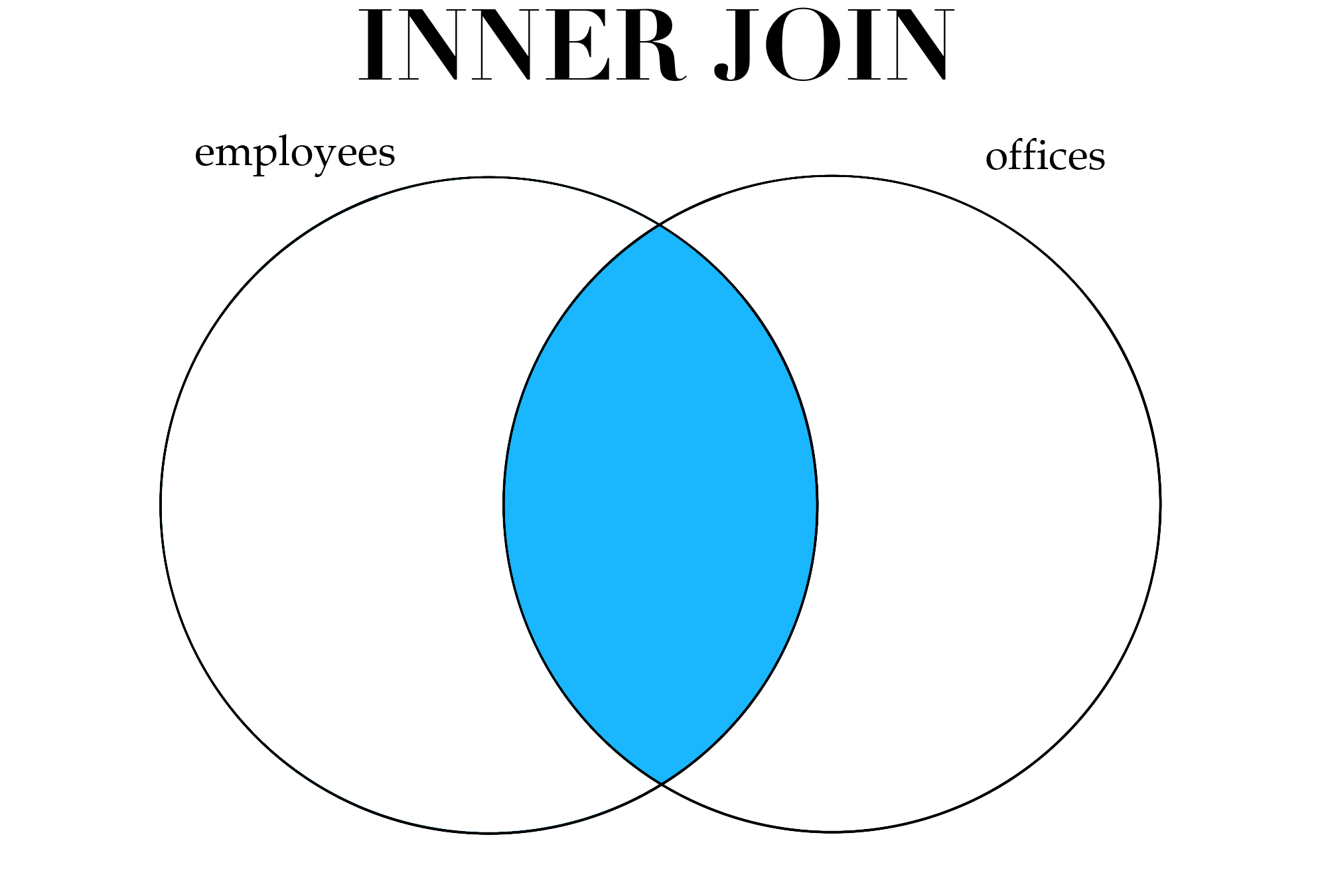
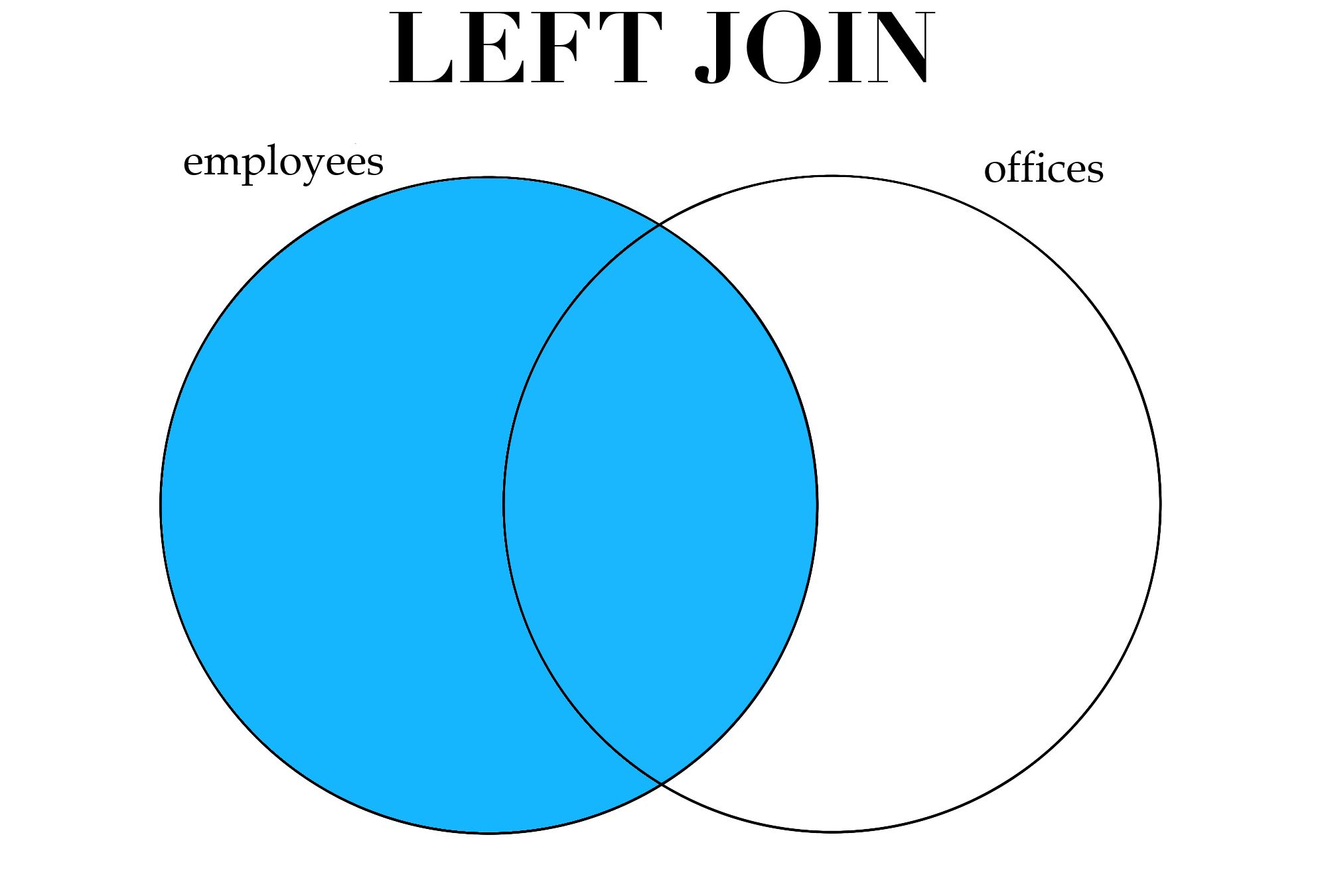
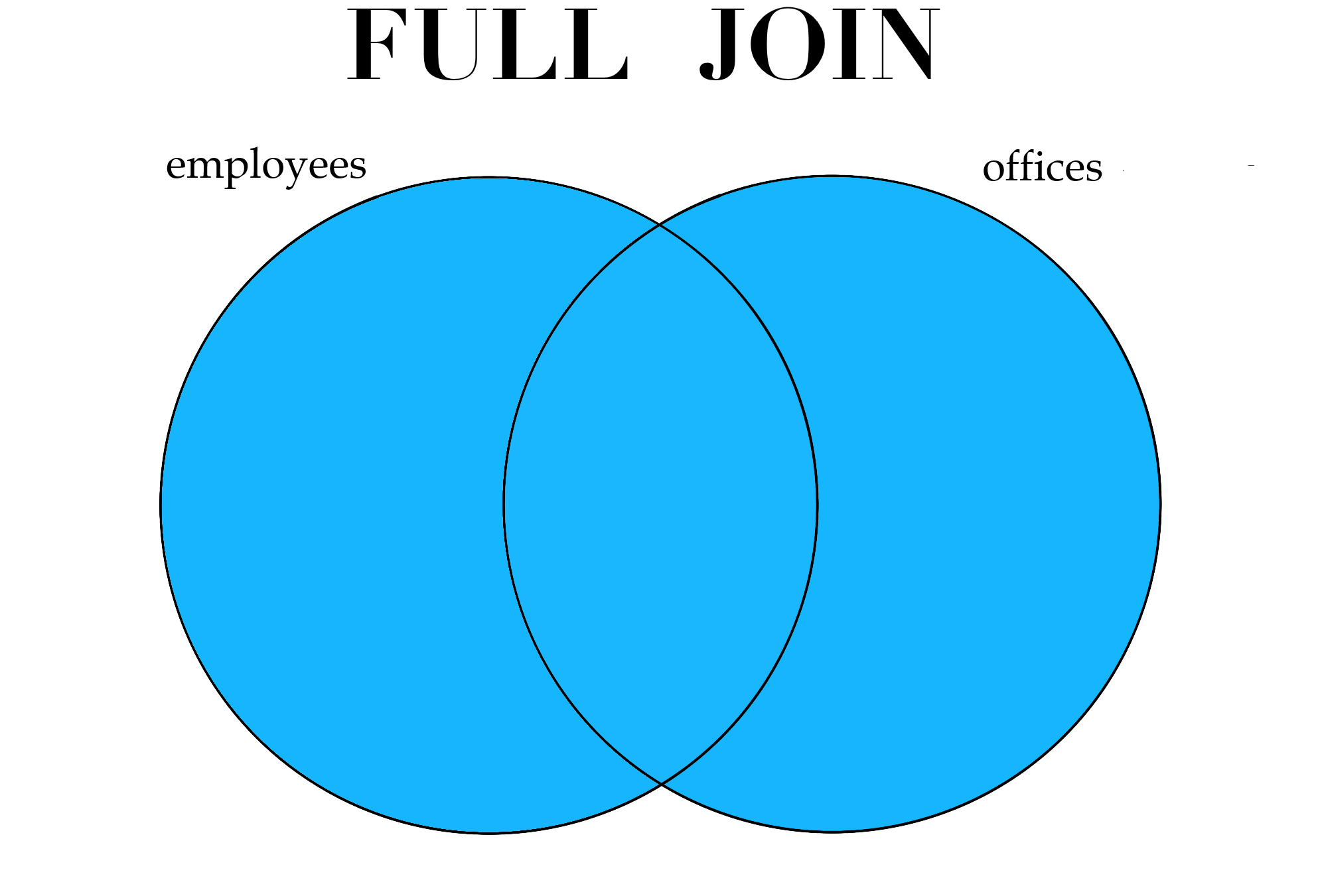
Figure 3.1: Different types of joins.
These types of joins can be performed in R with the following functions, which take the same arguments:
tidyverse::inner_join(df1, df2, by=NULL, suffix=c(“.x”, “.y”))
tidyverse::left_join(df1, df2, by=NULL, suffix=c(“.x”, “.y”))
tidyverse::full_join(df1, df2, by=NULL, suffix=c(“.x”, “.y”))
- Required arguments
- The two data frames to join together (
df1anddf2).
- The two data frames to join together (
- Optional arguments
by: A character with the name of the variable to use as the key in the merge. In our example, we would setby="ID", becauseIDis the common key between the two data sets. Ifbyequals the default value ofNULL, the function will automatically join on all variables that have the same name in the two data frames.suffix: If the two data frames have a column with the same name, thesuffixvalues will be added to the common column names in the joined data set so that they can be distinguished.
Let’s use inner_join() to create a new data frame with columns from both employees and offices:
## # A tibble: 6 x 11
##      ID Name     Gender   Age Rating Degree   Start_Date Retired Division Salary
##   <dbl> <chr>    <chr>  <dbl>  <dbl> <chr>    <chr>      <lgl>   <chr>    <chr>
## 1  2671 Lewis, ~ Male      34      4 Ph.D     2/23/07    FALSE   Enginee~ $182,~
## 2  8925 el-Jaff~ Female    50     10 Master's 2/23/91    FALSE   Enginee~ $206,~
## 3  2769 Soto, M~ Male      52     10 High Sc~ 2/23/87    FALSE   Sales    $183,~
## 4  2658 al-Ebra~ Male      55      8 Ph.D     2/23/85    FALSE   Corpora~ $236,~
## 5  1933 Medina,~ Female    62      7 Associa~ 2/23/79    TRUE    Sales    <NA>
## 6  3570 Troftgr~ Female    47      8 High Sc~ 2/23/95    FALSE   Operati~ $101,~
## # ... with 1 more variable: office <chr>
Think carefully about the type of join you are performing.
It is always important to think carefully about the type of join one is performing, and which observations might be lost as a result of the join. In this case, we are performing an inner join, which means that our new data frame innerJoinData does not contain:
- Employees whose office location was missing from
offices. - Employees whose information was not recorded in
employees.
The particular context of an analysis is key in determing whether or not it is acceptable to drop certain observations in a join. Unfortunately it is easy to perform joins in R without fully thinking through which data might be lost. This can result in serious errors or skewed analyses, so one should always perform checks on the data after the join to make sure it contains the intended set of observations. For example, we might re-check the dimensions of our data to see how they have changed after the join:
## [1] 908 11There are 90 employees in the data set who are not represented in offices, so we would expect 910 rows (i.e., 1,000 - 90 = 910) in our new data. However, if we had believed that all employees were represented in both data sets this would raise some concerns, as we would expect our joined data to have 1,000 rows.
So how can we compare the average salary of employees across the three different offices using innerJoinData? That question will be answered in the next chapter, which covers exploring and summarizing data.
References
Wickham, Hadley, and Jennifer Bryan. 2019. Readxl: Read Excel Files. https://CRAN.R-project.org/package=readxl.