Chapter 2 The Basics of R
When you work with data in Excel, each value in your data set is stored in an individual cell, and each one of those cells has a unique name made up of a letter and a number. For example, in the figure below, cell A1 stores the value “1”, cell B3 stores the value “learning”, cell C2 stores the value “2/26/2021”, etc.
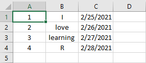
Figure 2.1: Example Excel Worksheet.
Once you have data stored in cells, you can apply formulas to those cells by referencing the cell names. For example, if you ran =SUM(A1:A4), Excel would sum the values stored in cells A1 through A4 and evaluate to 10 (i.e., 1 + 2 + 3 + 4 = 10). If this example is framiliar to you, you already understand the basics of R programming! Below we will see how this example translates into R code.
To learn how to program in R, you do not need a complete understanding of how the language is designed. However, you should know that everything you create in an R program is referred to as an object. Every object you create belongs to one of several classes, which determines the properties and attributes of the object.
To see what this means in concrete terms, let’s take a look at some R code. In the code below, we create an object called A1, which contains the value 1. We can create objects (or variables) with the assignment operator <-. When we run this line of code, we create an object called A1 that stores the value 1. Think of this as similar to entering the value 1 into cell A1 in an Excel worksheet.
Note that this code does not produce any output; all we are doing is storing the value 1 in a variable called A1, so there are no results to print out.
If we want to see what’s stored in our variable, we can simply run a line of code with the name of the variable and R will output its contents.
## [1] 1Now let’s observe the class of our object. To do this, we will use one of R’s built-in functions. In general terms, functions accept inputs (referred to as arguments), process them in some way, and then produce outputs. The class() function takes an object as an input and outputs the class of that object.
class(object_name)
Below, we pass our A1 object into the class() function to observe A1’s class.
## [1] "numeric"From this output we can see that our object A1 is a "numeric", which means it stores a number. Note that we did not need to explicitly tell R which class A1 should belong to - because we were storing a number in A1, R automatically knew to create a "numeric" object.
We can name our variables anything we want, subject to two rules:
- A variable name has to start with a letter and can contain letters, numbers, underscores, and periods.
- A variable cannot have the same name as any of R’s reserved words. These are words that already have meaning in the R language. For example, we could not create a variable called
class, because this word is already being used for theclass()function.
Below we create some more variables.
## [1] 5.5## [1] "I love IDS."## [1] 9Finally, let’s recreate our Excel example in R. Like Excel, R has a built-in sum() function that we can use to add up values.
sum(value1, value2, value3, …)
Unlike Excel, we need to list each variable individually instead of using A1:A4. Note also that because we already created A1 above, we do not need to create it again.
## [1] 10So far we have only created variables that store single values. However, because data comes in many different forms, there are many different types of objects you can create in R. In sections 2.2 and 2.3, we explore many of the different data types and data structures that you need to be framiliar with to work with data in R. First, however, we need to give a brief overview of the building blocks of data.
2.1 The Building Blocks of Data
Anyone who is familiar with Excel is framiliar with the basic shape of structured data. Data is typically displayed in a table, with multiple rows and columns. For example, below we have a data set with information on 1,000 employees from a software company. (For convenience we only display the first six rows of the data set.)
By convention, the observations (i.e., the employees) form the rows of the data set, and the variables (i.e., the characteristics of the employees we are measuring) form the columns. The dimensions of the data set are typically written as \(n\) x \(m\), where \(n\) is the number of observations (or rows) and \(m\) is the number of variables (or columns).
| ID | Name | Gender | Age | Rating | Degree | Start_Date | Retired | Division | Salary |
|---|---|---|---|---|---|---|---|---|---|
| 6881 | al-Rahimi, Tayyiba | Female | 51 | 10 | High School | 2/23/90 | FALSE | Operations | $108,804 |
| 2671 | Lewis, Austin | Male | 34 | 4 | Ph.D | 2/23/07 | FALSE | Engineering | $182,343 |
| 8925 | el-Jaffer, Manaal | Female | 50 | 10 | Master’s | 2/23/91 | FALSE | Engineering | $206,770 |
| 2769 | Soto, Michael | Male | 52 | 10 | High School | 2/23/87 | FALSE | Sales | $183,407 |
| 2658 | al-Ebrahimi, Mamoon | Male | 55 | 8 | Ph.D | 2/23/85 | FALSE | Corporate | $236,240 |
| 1933 | Medina, Brandy | Female | 62 | 7 | Associate’s | 2/23/79 | TRUE | Sales |
As we will see in Section 2.3.4, data sets like the one above are stored in R as data frames. However, before we get to a full-fledged data frame, we need to first understand the building blocks of data in R. We could break our data frame down by looking at a specific column, or a specific row. For example, we might want to look at just the Name column:
| Name |
|---|
| al-Rahimi, Tayyiba |
| Lewis, Austin |
| el-Jaffer, Manaal |
| Soto, Michael |
| al-Ebrahimi, Mamoon |
| Medina, Brandy |
Now instead of a full data frame we have a single set of values, i.e. the list of everyone’s names. In R we can store this type of data in either an atomic vector or a list, which we’ll learn about in Sections 2.3.1 and 2.3.3. But we can break this down even further! Image we want to look at a single value, for example the first name in our list:
## [1] "al-Rahimi, Tayyiba"Now we have a single value. This particular observation is text, but it could also be a number, a date, a Boolean value (i.e., TRUE/FALSE), etc. From this example we can start to see how full data sets in R are constructed.The smallest unit of data are single values, which can be combined to form vectors (or lists), which can be combined to form data frames (or matrices). The following two sections (2.2 and 2.3) walk through these building blocks in more detail.
2.2 Data Types
You are likely framiliar with the window below from Excel, which shows the format of a cell (or group of cells). The proper choice of format depends on the type of data contained in the cell. For example, a column containing customers’ names should be formatted as General or Text; a column with the transaction dates of customer orders should be formatted as Date; a column with sales prices should be formatted as Currency or Accounting.
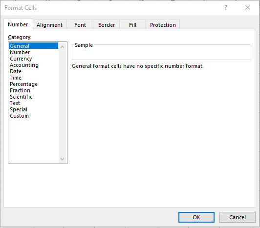
Figure 2.2: The Format Cells Window in Excel.
Just like Excel, R has several data types that specify the type of data you are working with. The following are the primary data types that you should be aware of:
Logical - Used to store Boolean data, which only take on the values
TRUEorFALSE. For example, the employee data contains a variable calledretiredthat equalsTRUEif the employee is retired andFALSEif they are not retired.## [1] "logical"Numeric - Used to store numbers with or without values after the decimal. The
age,performance,seniority, andincomevariables in the employee data are all stored as numerics.## [1] "numeric"Character - Used to store text data, in particular text variables that can take on an infinite or very large set of possible values. For example, employee names, which could be nearly anything, should be stored as a character.
## [1] "character"- Factor - Used to represent categorical variables that take on a fixed set of values. For example, the
Degreevariable in the employee data can only take on five possible values:High School,Associate's,Bachelor's,Master's, andPh.D. Therefore, one would likely want to store this variable as a factor.Note that it can often be difficult to decide whether something should be stored as a factor or a character. It is possible to store
departmentas a character instead of as a factor, and in many circumstances this would not be an issue. However, there are certain circumstances where you want R to recognize that a variable takes on a limited set of values. We will see this later in Section 6 when we discuss the use of dummy variables in regression.## [1] "factor"
Date - Used to store dates in R.
## [1] "Date"NA - Used to represent missing data in R. We often work with data sets that have missing values. For example, in our employees data set, we do not know the
Salaryof some of the employees. In Excel we might represent this with#N/A, but in R it would be stored asNA. Because missing data is such a common issue, we will revisitNAfrequently throughout this book. One has to be particularly careful with missing data in R, asNAvalues can create issues and unexpected behaviors that are sometimes difficult to detect.
2.3 Data Structures
Now that we know the types of data we can store in R, let’s explore the different data structures that we can use to store those data. The majority of the analyses shown in this book will be based around data frames, and we will also rely heavily on atomic vectors. We will use matrices and lists much less frequently.
2.3.1 Atomic Vectors
Perhaps the most basic data structure in R is the atomic vector, which stores a set of one or more values of the same type. There are two important components to this definition:
- Atomic vectors can store one or more values, meaning an object that stores just a single value is an atomic vector. This means that every object we have created so far (e.g.,
A1in Section 2) has been an atomic vector. Below we will see how to create atomic vectors with more than one value. - Atomic vectors cannot mix data types. This means you could not have an atomic vector with numbers and characters, for example.
As we’ve seen throughout the book so far, single-value atomic vectors can be created by simply assigning a value to a variable:
v1 <- 2             # Numeric atomic vector
v2 <- TRUE          # Logical atomic vector
v3 <- "R is fun!"   # Character atomic vector
If we want to combine multiple values into a single atomic vector, we need to use the c() command, which stands for “combine”:
v4 <- c(2, 3, 4, 5)                 # Numeric atomic vector
v5 <- c(TRUE, TRUE, FALSE)          # Logical atomic vector
v6 <- c("R is fun!", "I hate R")    # Character atomic vector
v7 <- c(8, 9, 10, NA)               # Numeric atomic vector with missing value
Now that we have multiple values stored in a single atomic vector, there are many different functions we can apply to these atomic vectors. This is equivalent to applying an Excel function to a series of cells. For example:
length(vectorName)
Returns the number of elements in the atomic vector called vectorName.
## [1] 4## [1] 3## [1] 2## [1] 4sum(vectorName, na.rm=FALSE)
- Required arguments
- The atomic vector whose values one would like to sum.
- Optional arguments
na.rm: IfTRUE, the function will remove any missing values (NAs) in the atomic vector and sum the non-missing values. IfFALSE, the function does not removeNAs and will return a value ofNAif there is anNAin the atomic vector.
Note that this will not work for v6, because there is no logical way to sum characters together. If we apply it to v5, it will treat the TRUE values like 1 and the FALSE values like 0.
## [1] 14## [1] 2Now let’s try applying it to v7, which has a missing value:
## [1] NABecause the default value of na.rm is FALSE, the function does not remove the NA from v7, and returns NA. If we explicitly set na.rm to TRUE, the function will return the sum of the non-missing values:
## [1] 27mean(vectorName, na.rm=FALSE)
- Required arguments
- The atomic vector whose values one would like to average.
- Optional arguments
na.rm: IfTRUE, the function will remove any missing values (NAs) in the atomic vector and average the non-missing values. IfFALSE, the function does not removeNAs and will return a value ofNAif there is anNAin the atomic vector.
## [1] 3.5## [1] 0.6666667As with sum(), the function returns NA for v7 if we fail to change the na.rm argument:
## [1] NAIf we set the argument to TRUE, we get the average of the non-missing values in v7.
## [1] 9min(vectorName, na.rm=FALSE) and max(vectorName, na.rm=FALSE)
- Required arguments
- The atomic vector whose values one would like to find the minimum/maximum of.
- Optional arguments
na.rm: IfTRUE, the function will remove any missing values (NAs) in the atomic vector and find the minimum/maximum of the non-missing values. IfFALSE, the function does not removeNAs and will return a value ofNAif there is anNAin the atomic vector.
## [1] 2## [1] 5## [1] 8## [1] 102.3.2 Matrices
Whereas atomic vectors are one-dimensional, a matrix can be used to store two-dimensional data in R. However, like atomic vectors, matrices can only store values of the same type. This means that we could not store the employee data in a matrix, because that data set contains a mix of numeric, character, and factor variables. Although we describe matrices here so the reader is aware of them, we will not rely on them heavily throughout the rest of the book.
We can create a simple matrix in R with the matrix() function, which uses the following syntax:
matrix(data, nrow, ncol)
- Required arguments
datais a vector with the values we want to fill the matrix
- Optional arguments
nrowis the desired number of rows of the matrixncolis the desired number of columns
For example:
matrixData = c(1,2,3,4,5,6,7,8,9)         # Define values that will fill the matrix
matrixExample = matrix(matrixData, 3, 3)  # Create matrix
matrixExample
## [,1] [,2] [,3]
## [1,] 1 4 7
## [2,] 2 5 8
## [3,] 3 6 92.3.3 Lists
Lists are similar to atomic vectors, except that a single list can store elements of different types. We can create lists with the list() function:
list(object1, object2, object3, …)
l1 <- list(2, TRUE, "Lists!", 5.5)
l2 <- list(c(1, 2, 3), c(TRUE, FALSE, TRUE), c("my", "second", "list"))
l3 <- list(l1, l2)
The first list we create, l1, contains a mix of numeric, logical, and character values. When we output the contents of this list, we see the following:
## [[1]]
## [1] 2
##
## [[2]]
## [1] TRUE
##
## [[3]]
## [1] "Lists!"
##
## [[4]]
## [1] 5.5
The double-brackets (“[[" and "]]”) tell us the position of each value in the list; the value 2 is the first element in the list, the value TRUE is the second element, etc. We can extract a specific value from a list by referencing its index with these double-brackets:
## [1] 2The second list we create, l2, is slightly more complicated. This time, each element of the list is actually an atomic vector. We can see this when we output the contents of the list:
## [[1]]
## [1] 1 2 3
##
## [[2]]
## [1]  TRUE FALSE  TRUE
##
## [[3]]
## [1] "my"     "second" "list"
Now the first element in the list is the atomic vector c(1, 2, 3), the second element is the atomic vector c(TRUE, FALSE, TRUE), etc.
Finally, our last list is actually a list of our first two lists! Lists are called recursive because they can contain other lists. See if you can parse the output of l3:
## [[1]]
## [[1]][[1]]
## [1] 2
##
## [[1]][[2]]
## [1] TRUE
##
## [[1]][[3]]
## [1] "Lists!"
##
## [[1]][[4]]
## [1] 5.5
##
##
## [[2]]
## [[2]][[1]]
## [1] 1 2 3
##
## [[2]][[2]]
## [1]  TRUE FALSE  TRUE
##
## [[2]][[3]]
## [1] "my"     "second" "list"
As before, we can use double-brackets to extract individual values in the list:
## [[1]]
## [1] 2
##
## [[2]]
## [1] TRUE
##
## [[3]]
## [1] "Lists!"
##
## [[4]]
## [1] 5.5
This time, because the first element in l3 is itself a list, we can add a second set of double-brackets to get an individual element from this second list:
## [1] "Lists!"2.3.4 Data Frames
Now we are ready for the primary data structure that is used to handle full data sets in R: the data frame. Data frames are two-dimensional objects that can store values of different types. This distinguishes them from matrices, which can only store values of a single type. Behind the scenes, a data frame is actually just a list of vectors; each column is a vector, and those vectors are combined in a list to form a data frame.
The employee data set that we saw in Section 2.1 is an example of a data frame. The next chapter of this book, Chapter 3, will focus entirely on data frames and how you can use them to organize and manipulate data sets in R.
You may recall from Section 1.2.1 that throughout this book, we will be relying on a collection of packages known as the tidyverse. The foundation of the tidyverse packages is a tweaked form of the traditional data frame known as a tibble. Tibbles are essentially data frames, but with some of the functionality changed to make data processing simpler and more efficient. Throughout the book we will refer to our data sets by the term “data frame”, but technically they will be stored as tibbles.