Chapter 9 Supervised Machine Learning: Additional Algorithms

In the previous chapter we presented a single machine learning model (the kNN algorithm), and demonstrated how this algorithm can be used in the context of a supervised machine learning problem. In this chapter, we will explore additional algorithms that are commonly used in industry for supervised machine learning. All of the principles that we covered in the context of kNN (the bias-variance tradeoff, cross validation, etc.) apply to the algorithms in this chapter as well.

9.1 Regularized Regression Models

As discussed in Section 8.2, statistical modeling can be used for either prediction or inference. In Chapter 6, we covered linear and logistic regression from an inference perspective, where our primary goal was to understand how variables related to one another. In this Chapter, our focus is instead on prediction. When prediction is the primary aim, a process known as regularization is often applied to linear or logistic regression models to improve their predictive ability.

Additionally, the regression models we learned about in Chapter 6 do not perform well when the independent ($X$) features are highly correlated (a problem known as multicollinearity, see 6.1.6.2), and these models fail to provide any estimates at all when the number of independent features exceeds the number of observations. These problems can also be addressed through regularized regression models (also referred to as penalized regression models).

The idea behind regularization is that we impose a constraint on the coefficients of the regression model. This constraint can push the coefficients of irrelevant features towards zero, or drive them all the way to zero. This can result in more accurate models that (in some cases) are easier to interpret. Although the constraint results in a model that has a worse fit to the training data, in some cases the resulting model generalizes better to unseen data. This is because the constraint on the coefficients can prevent the model from overfitting the training data. We need to optimize the size of the constraint in order to balance this bias variance tradeoff (discussed in Section 8.4).

Note that regularization can be applied to both linear and logistic regression. There are three common regularized models we can implement: lasso, ridge, and elastic net.

9.1.1 Ridge

[In Progress]

9.1.2 Lasso

[In Progress]

9.1.3 Elastic Net

[In Progress]

9.2 CART Models

Classification and regression tree (CART) models are a popular class of machine learning algorithms that make predictions according to a set of logical rules learned from training data. Tree models that predict discrete outcomes are referred to as classification trees, while tree models that predict continuous outcomes are referred to as regression trees.

One major advantage of CART models is their interpretability. As we will see, CART models make predictions according to a series of logical rules that can be analyzed and understood by human users. This is in contrast to many other algorithms (like the random forest model discussed in the next section), which are more difficult to interpret.

9.2.1 Classification Trees

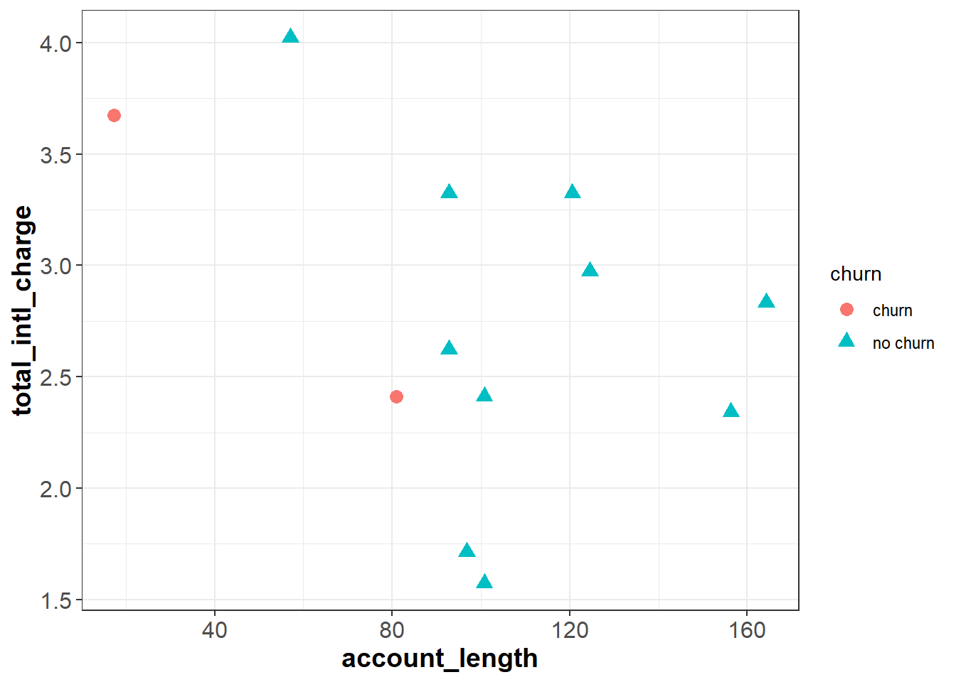
To understand classification trees, let’s start with a simplified version of our churn data set that only has twelve observations and two independent features, total_intl_charge and account_length. Our feature space looks as follows:

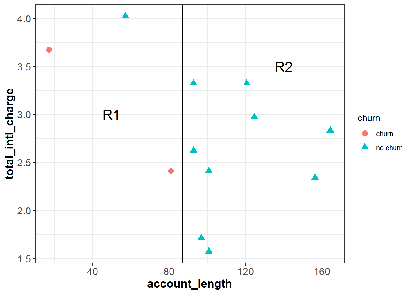
The classification tree algorithm works by drawing a straight line that partitions the feature space to maximize the homogeneity (or minimize the entropy) of each sub-region. For example, imagine we drew a vertical line at around account_length = 87, dividing the feature space into R1 and R2. Intuitively, R2 is completely homogeneous because it only contains observations with the same outcome—“no churn”. R1 is less homogeneous because it contains two “churn” observations and one “no churn” observation.

In this simple example we made cuts based on a visual inspection of the data, but the classification tree algorithm uses a measure known as entropy to ensure that each cut maximizes the homogeneity of the resulting subspaces. Entropy is defined as follows:

\[Entropy = -\sum_i^C{p_ilog(p_i)}\]

where the data set has $C$ classes (or unique outcome values), and $p_i$ represents the proportion of observations in the data from the $i$th class. In our case $C=2$ because we have two classes: “churn” and “no churn”. Notice, this is very similar to the log loss formula that we introduced in Section 8.5.1.3.

Using this formula, we can first calculate the entropy of our original data set (before we made any cuts), which we’ll call $E_0$. There are two “churn” customers and ten “no churn” customers, so the entropy is:

\[E_0 = -[\frac{2}{12}log(\frac{2}{12}) + \frac{10}{12}log(\frac{10}{12})] = 0.1957\]

Now we will calculate the entropy after making the cut, for each subspace separately. The subspace R2 is completely homogeneous (all nine customers are “no churn”), so the entropy equals zero:

\[E_{R2} = -[\frac{9}{9}log(\frac{9}{9})] = 0\]

The subspace $R1$ has one “no churn” and two “churns”, so the entropy equals:

\[E_{R1} = -[\frac{2}{3}log(\frac{2}{3}) + \frac{1}{3}log(\frac{1}{3})] = 0.2764\]

To calculate the overall entropy after making the cut at account_length = 87, we take a weighted average of $E_{R1}$ and $E_{R2}$ based on the number of observations in each subspace:

\[E_{Cut1} = \frac{3}{12}E_{R1} + \frac{9}{12}E_{R2} = 0.0691\]

The information gain, or the reduction in entropy due to this cut, is then: \[E_0 - E_{Cut1} = 0.1957 - 0.0691 = 0.1266\]

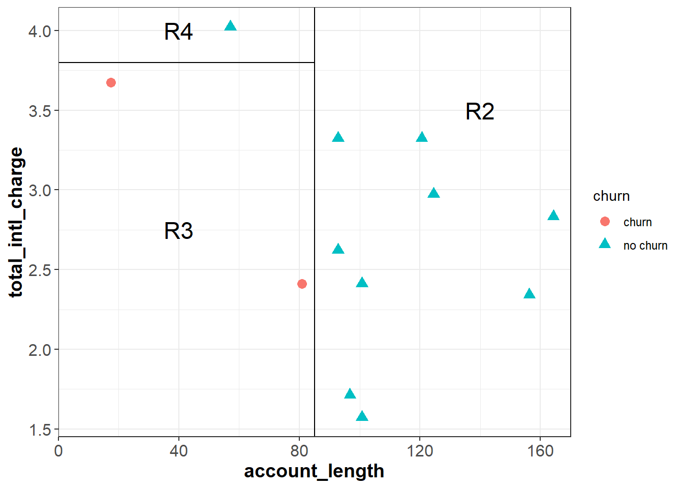
Each cut is made at the point that will result in the greatest reduction in the information gain. To further reduce the entropy of R1, we can make a cut around total_intl_charge = 3.8 to partition R1 into two smaller regions (R3 and R4) that are completely homogeneous. Because the feature space is completely divided into pure regions, the entropy after the second cut is zero:

\[\begin{aligned}E_{Cut2} & = \frac{9}{12}E_{R2} + \frac{2}{12}E_{R3} + \frac{1}{12}E_{R4} \\ & = \frac{9}{12}(0) + \frac{2}{12}(0) + \frac{1}{12}(0) \\ & = 0 \end{aligned}\]

Because each subspace is completely pure, there are no additional cuts we could make to further reduce the entropy.

To create pure feature space, we first made a cut at account_length = 87, then within the region where account_length was less than 87 made an additional cut at total_intl_charge = 3.8. From this we can write out a set of decision rules:

We can use this decision tree to predict whether or not a new observation will churn. For example:

If a new observation has an account_length greater than or equal to 87, we move down the left branch of the tree and predict “no churn”.
If a new observation has an account_length less than 87 and a total_intl_charge greater than or equal to 3.8, we would move right at the first split and left at the second split of the tree, leading to a prediction of “no churn”.
If a new observation has an account_length less than 87 and a total_intl_charge less than 3.8, we would move right at the first split and right at the second split of the tree, leading to a prediction of “churn”.

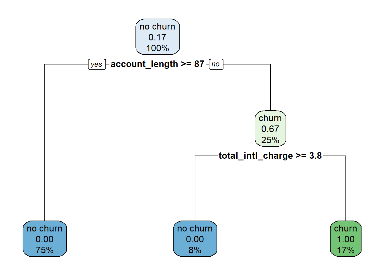
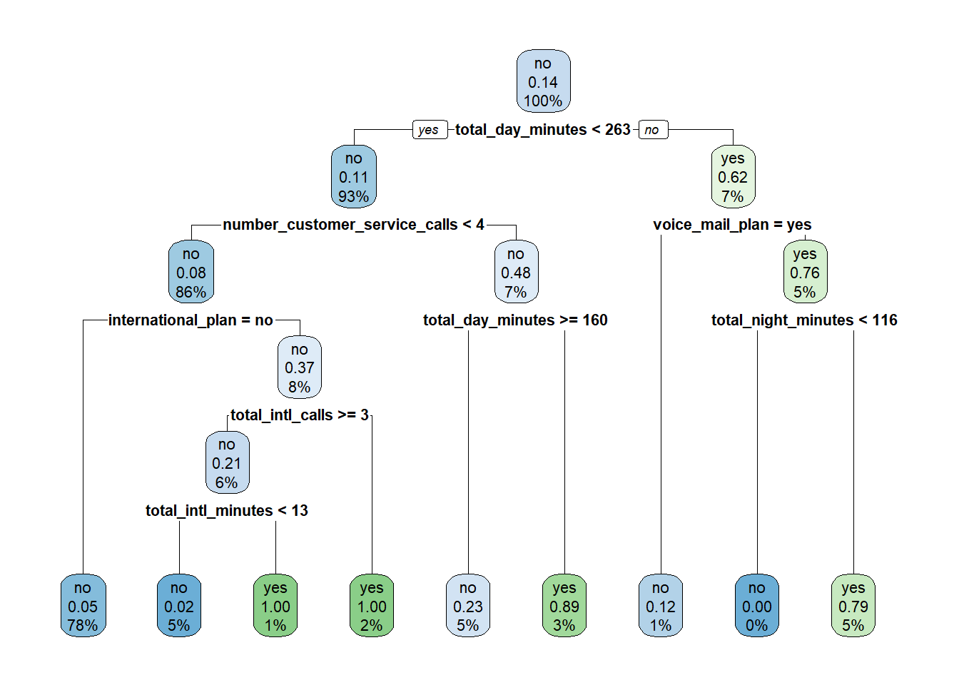
How do we interpret the numbers shown in the tree? In the plot each node has three rows, showing (in order):

The majority class in that node (“churn” / “no churn”).
The proportion of the observations in that node that churned.
The percentage of the total data inside that node.

For example, let’s start at the top node, which represents the data set before any cuts have been made. Because no cuts have been made, this node includes all of the data, so the third line shows 100%. Of the twelve observations in the data set, two of them churned, so the proportion of observations that churned equals (2 / 12) $\approx$ 0.17. Because this proportion is lower than the default cutoff of 0.5, the majority class for this node is “no churn”.

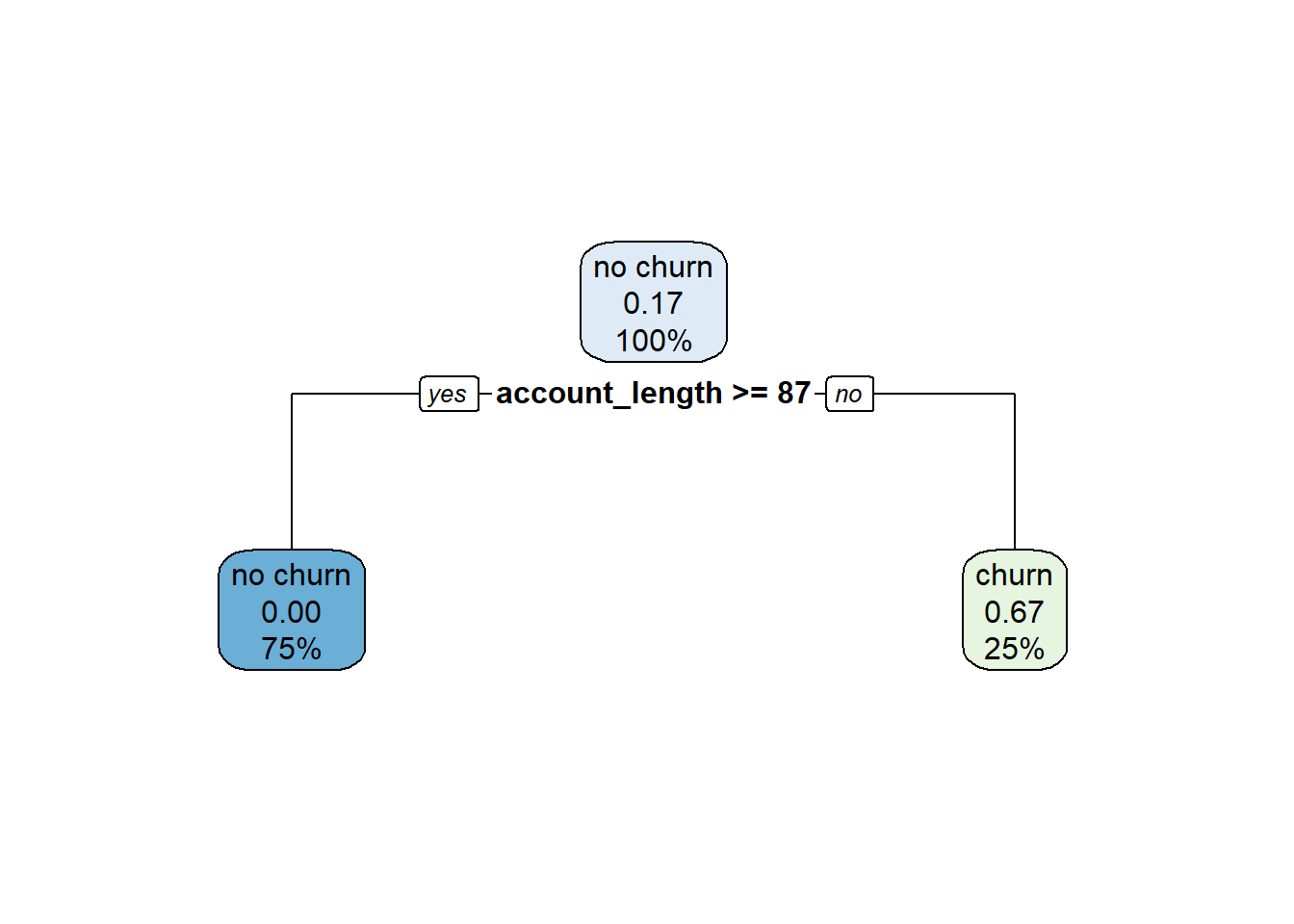
Now imagine what happens as we work our way down the tree. If account_length is greater than or equal to 87 we move to the left branch. This corresponds to the subspace R2 in the plot of the feature space. This subspace contains nine observations, or 75% of the total observations in the data set ((9 / 12) = 75%). None of these observations churned, so the second line in the node is 0.00, and the majority class is “no churn”.

Now imagine we work our way down the right branch of the tree. If account_length is less than 87, we move into the subspace R1. R1 has three observations ((3 / 12) = 25%), two of which churned ((2 / 3) $\approx$ 0.67). From this node, if total_intl_charge is less than 3.8 we move to the right, which represents subspace R3. Here we have two observations ((2 / 12) $\approx$ 17%), both of which churned ((2 / 2) = 1.00). If instead total_intl_charge is greater than or equal to 3.8 we move to the left, which represents subspace R4. Here we have one observation ((1 / 12) $\approx$ 8%), which did not churn ((0 / 1) = 0.00).

In R, we can fit a classification tree to our data using the rpart() function from the rpart package. This function uses the following syntax:

rpart::rpart(y ~ x1 + x2 + … + xp, data, maxdepth=30)

Required arguments
- y: The name of the dependent ($Y$) variable.
- x1, x2, … xp: The name of the first, second, and $pth$ independent variables.
- data: The name of the data frame with the y, x1, x2, and xp variables.
Optional arguments
- maxdepth: The maximum depth of the tree (see Section ??).

Then, after we have built a model with rpart(), we can visualize the tree with the rpart.plot() function from the rpart.plot package:

rpart.plot::rpart.plot(x)

Required arguments
- x: A tree model built with rpart().

Below we apply these functions to our full churn data set:

model <- rpart(churn ~ ., data=churn)
rpart.plot(model)

9.2.1.1 Tuning Hyperparameters

Let’s return to the simplified data set from the previous section, with only twelve observations and two features. After inspecting the classification tree we built from this data, you may suspect that something is wrong with the right branch - customers with a higher total_intl_charge are classified as “no churn”, while customers with a lower total_intl_charge are classified as “churn”. Based on the context of the business we may find this pattern surprising, as we expect customers with high international charges to be more likely to switch services. One possibility is that we are overfitting the data, so the decision tree is picking up on the noise in the sample instead of the signal.

To prevent overfitting, we can prune the decision tree to a certain depth; or, in other words, limit how many cuts we can perform. For example, let us prune this tree to a depth of one, meaning the algorithm cannot make more than one cut. The resulting pruned tree is shown below. Under this set of rules, customers with an account_length greater than or equal to 87 are classified as “no churn”; this is because subspace R2 (which represents account_length >= 87) contains only “no churn” observations. Customers with an account_length less than 87 are assigned a probability of churning of 0.67; this is because subspace R1 (which represents account_length < 87) contains two “churn” observations and one “no churn” observation ((2 / 3) $\approx$ 0.67).

For CART models, the depth hyperparameter serves a similar purpose as the $k_{knn}$ hyperparameter for the kNN algorithm. By tuning the value of the tree’s depth, we seek to balance the bias-variance tradeoff. If the depth is too large, our tree will grow too deep and overfit the training data. Conversely, if the depth is too small, our tree will not grow deep enough and will underfit the training data. Therefore, we need to use cross validation to identify the value of depth that balances this tradeoff on our data.

In R, we can tune the depth hyperparameter through cross validation using the exact same functions shown in the previous chapter. To train a cross-validated classification tree, we can use the train() function from the caret package just as we did in the previous chapter (Section 8.4.2). To apply this function with the classification tree algorithm:

As before, we specify the independent and dependent variables in our model using the tilde (~). Remember that if you just replace the names of the features with the wildcard character ., the model will be built using all of the features in the data set.
Because the classification tree algorithm does not require the data to be normalized like kNN, we can pass in the data set churn instead of churnScaled.
To apply the classification tree algorithm, we set the method argument equal to "rpart2".
Recall that in Section @ref($k$-fold-cross-validation) we created an object called cvConditions, which is used to ensure that for each model we test, the cross validation process is performed consistently. We can re-use that object here so we can directly compare these results to the results from the kNN model.

By default, the train() function comes up with a grid of different hyperparameter values to test.

set.seed(972945)
rpartCV <- train(churn ~ ., 
                 data = churn,
                 method = "rpart2", 
                 trControl = cvConditions)

rpartCV

## CART 
## 
## 3400 samples
##   12 predictor
##    2 classes: 'no', 'yes' 
## 
## No pre-processing
## Resampling: Cross-Validated (5 fold) 
## Summary of sample sizes: 2720, 2720, 2719, 2720, 2721 
## Resampling results across tuning parameters:
## 
##   maxdepth  Accuracy   Kappa    
##   1         0.8720613  0.3290213
##   2         0.8823554  0.3917376
##   4         0.9161777  0.5991045
## 
## Accuracy was used to select the optimal model using the largest value.
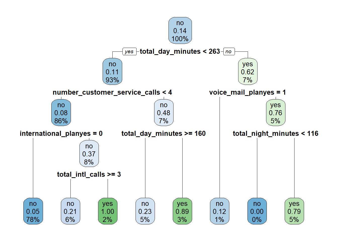
## The final value used for the model was maxdepth = 4.

Based on these results the optimal value of maxdepth is four, so our final tree will be pruned to a depth of four. We can visualize this tree by applying the rpart.plot() function to rpartCV$finalModel:

rpart.plot(rpartCV$finalModel)

9.2.2 Regression Trees

[In Progress]

9.3 Random Forest

One shortcoming of the CART model discussed in the previous section is that it typically exhibits high variance. This means that the model might change significantly if it were built on a different sample of data. In general we hope that our models are robust, and not highly dependent on the particular observations in the training set. Instead we prefer models that exhibit low variance, meaning the model parameters would not change drastically if we built the model on a different random sample of data.

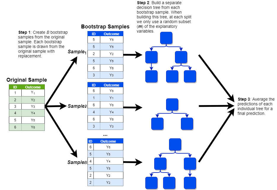
Statistical theory tells us that even if the variance of an individual model is high, the variance of many such models averaged together will be significantly lower. Of course, we usually only have one training set, so we do not have the luxury of building many different CART models on separate data sets and averaging them together. However, thanks to a technique known as bootstrapping, there is a way to build many different trees on a single data set. This model, known as the random forest, works according to the following steps:

Generate $B$ replicates of the training data by randomly sampling from the training data with replacement. Each replicate should be the same size as the original data set.
- Drawing a sample with replacement means that a given observation can be included multiple times in the sample. Imagine that we were randomly drawing a sample of bingo balls out of a hat. If we drew G7, we would record that value in our sample and then throw it back into the hat before drawing the next ball. This implies that we could potentially draw G7 again later on.
- This process is called bootstrapping.
Build separate decision trees on each of the $B$ samples, with one caveat. Instead of freely building the decision trees, there is one additional rule: each time we make a cut, consider only a random subset of $m$ features from the full set of $p$ features; a common rule of thumb is that $m$ should be around the square root of $p$.
- In this example, we are training a random forest to predict churn using the twelve independent features in our data set (so $p$ = 12). As the square root of twelve is 3.46, let’s think through the random forest model with an $m$ of four. Each individual tree in our forest is built on one of the $B$ independent samples that were drawn in the previous step. Every time a cut is made within each of these trees, the algorithm randomly selects four of the twelve independent features in our data set. As before, the cut is made based on whichever one of these four features minimizes the entropy (i.e., maximizes the information gain). For the next cut, another set of four features are randomly selected, and the process is repeated.
Make predictions for new observations by averaging the predictions of all of the trees together.

This process is shown in the visualization below (with a simplified sample of only six observations):

We can fit a random forest model in R with the randomForest() function from the randomForest package, which uses the following syntax:

randomForest::randomForest(y ~ x1 + x2 + … + xp, data, ntree=500, mtry, importance=FALSE)

Required arguments
- y: The name of the dependent ($Y$) variable. If this variable is coded as a factor the model assumes you are trying to perform classification; if it is coded as a numeric, the model assumes you are trying to perform regression.
- x1, x2, … xp: The name of the first, second, and $pth$ independent variables.
- data: The name of the data frame with the y, x1, x2, and xp variables.
Optional arguments
- ntree: The number of trees to build in the forest (i.e., the number of bootstrap samples $B$).
- mtry: The number of variables randomly sampled as candidates at each split ($m$). For classification, the default value is the square root of the number of independent features ($\sqrt{p}$). For regression, the default is the number of independent features divided by three ($p / 3$).
- importance: Whether the importance of the predictors should be assessed. By default this is FALSE, but we will set it to TRUE so that we can observe the importance of each feature in the next section.

Below we apply this to the churn data set:

modelRF <- randomForest(churn ~ ., data=churn, importance=TRUE)

9.3.1 Feature Importance

Because a random forest model is comprised of many, many individual trees, we cannot interpret it as easily as we did with the CART model in the previous section. With the classification tree we built, we could visualize the tree and understand how the model made predictions. This is not possible with a random forest model, as each prediction is a weighted average of (typically) hundreds of different trees. How, then, can we develop some sense of how the model makes predictions?

One method that has been developed for random forest models is variable importance, which attempts to measure the relative importance of each independent feature ($X$) in the model. Following the process described below, each independent feature is ranked according to how important that feature is in predicting the target feature ($Y$). This allows one to develop a sense for which information the model is relying on to make predictions.

Feature importance is calculated according to the following steps:

Calculate the Out-of-Bag (OOB) score for each tree in the forest.
- Remember that each tree in the forest is built on a bootstrap sample of the training data, which means each one of these samples is likely missing some of the observations from the training set. For example, in the visualization of the random forest in the previous section, the first bootstrap sample only contains observations 2, 3, 5, and 6; it does not contain observations 1 or 4. This means that for this sample, observations 1 and 4 are “out-of-bag” (i.e., not included). The OOB score for a tree is the prediction accuracy of that tree on its own out-of-bag observations. For the first tree, the OOB score is therefore the predictive accuracy of that tree on observations 1 and 4.
Randomly shuffle the values of the variable of interest. For example, if we were calculating the feature importance of total_day_minutes, we would randomly shuffle the total_day_minutes column in our data set. Then, re-calculate the OOB score for each tree as we did in Step 1, but now with one of the columns shuffled.
Calculate the final feature importance as the average difference between each tree’s two OOB scores, divided by the standard deviation of those differences.

Below we calculate the feature importance values for our model using the importance() function from the randomForest package, which uses the following syntax:

randomForest::importance(x, type=NULL)

Required arguments
- x: An model object created using randomForest().
Optional arguments
- type: Either 1 or 2, specifying the type of importance measure (1=mean decrease in accuracy, 2=mean decrease in node impurity). We will use type=1.

importance(modelRF, type=1)

##                               MeanDecreaseAccuracy
## account_length                           0.1154325
## international_plan                      88.7336548
## voice_mail_plan                         19.7810384
## number_vmail_messages                   17.5205295
## total_day_minutes                      104.9659477
## total_day_calls                         -0.7458680
## total_night_minutes                     10.6182409
## total_night_calls                        1.3900060
## total_intl_minutes                      32.7454747
## total_intl_calls                        49.5266029
## total_intl_charge                       31.4959813
## number_customer_service_calls           83.3429531

This output indicates that total_day_minutes is the most important predictive feature in the model, followed by international_plan, then number_customer_service_calls, etc.

9.3.2 Tuning Hyperparameters

For random forest we can use cross validation to tune the hyperparameter $m$, or the number of independent features randomly sampled as candidates at each split. As with the other models in this chapter, we can do this with the train() function from the caret package. Note that for random forest, we set method to "rf".

set.seed(972945)
rfCV <- train(churn ~ ., 
                 data = churn,
                 method = "rf", 
                 trControl = cvConditions)

rfCV

## Random Forest 
## 
## 3400 samples
##   12 predictor
##    2 classes: 'churn', 'no churn' 
## 
## No pre-processing
## Resampling: Cross-Validated (5 fold) 
## Summary of sample sizes: 2719, 2721, 2719, 2720, 2721 
## Resampling results across tuning parameters:
## 
##   mtry  Accuracy   Kappa    
##    2    0.9258848  0.6484207
##    7    0.9344173  0.7069461
##   12    0.9320622  0.6964866
## 
## Accuracy was used to select the optimal model using the largest value.
## The final value used for the model was mtry = 7.

9.4 XGBoost

[In Progress]