3.1 Review on parametric regression

We review now a couple of useful parametric regression models that will be used in the construction of nonparametric regression models.

3.1.1 Linear regression

Model formulation and least squares

The multiple linear regression employs multiple predictors $X_1,\ldots,X_p$ ⁹ for explaining a single response $Y$ by assuming that a linear relation of the form

$\begin{align} Y=\beta_0+\beta_1 X_1+\cdots+\beta_p X_p+\varepsilon \tag{3.1} \end{align}$

holds between the predictors $X_1,\ldots,X_p$ and the response $Y.$ In (3.1), $\beta_0$ is the intercept and $\beta_1,\ldots,\beta_p$ are the slopes, respectively. $\varepsilon$ is a random variable with mean zero and independent from $X_1,\ldots,X_p.$ Another way of looking at (3.1) is

$\begin{align} \mathbb{E}[Y|X_1=x_1,\ldots,X_p=x_p]=\beta_0+\beta_1x_1+\cdots+\beta_px_p, \tag{3.2} \end{align}$

since $\mathbb{E}[\varepsilon|X_1=x_1,\ldots,X_p=x_p]=0.$ Therefore, the mean of $Y$ is changing in a linear fashion with respect to the values of $X_1,\ldots,X_p.$ Hence the interpretation of the coefficients:

$\beta_0$ : is the mean of $Y$ when $X_1=\ldots=X_p=0.$
$\beta_j,$ $1\leq j\leq p$ : is the additive increment in mean of $Y$ for an increment of one unit in $X_j=x_j,$ provided that the remaining variables do not change.

Figure 3.1 illustrates the geometrical interpretation of a multiple linear model: a plane in the $(p+1)$ -dimensional space. If $p=1,$ the plane is the regression line for simple linear regression. If $p=2,$ then the plane can be visualized in a three-dimensional plot.

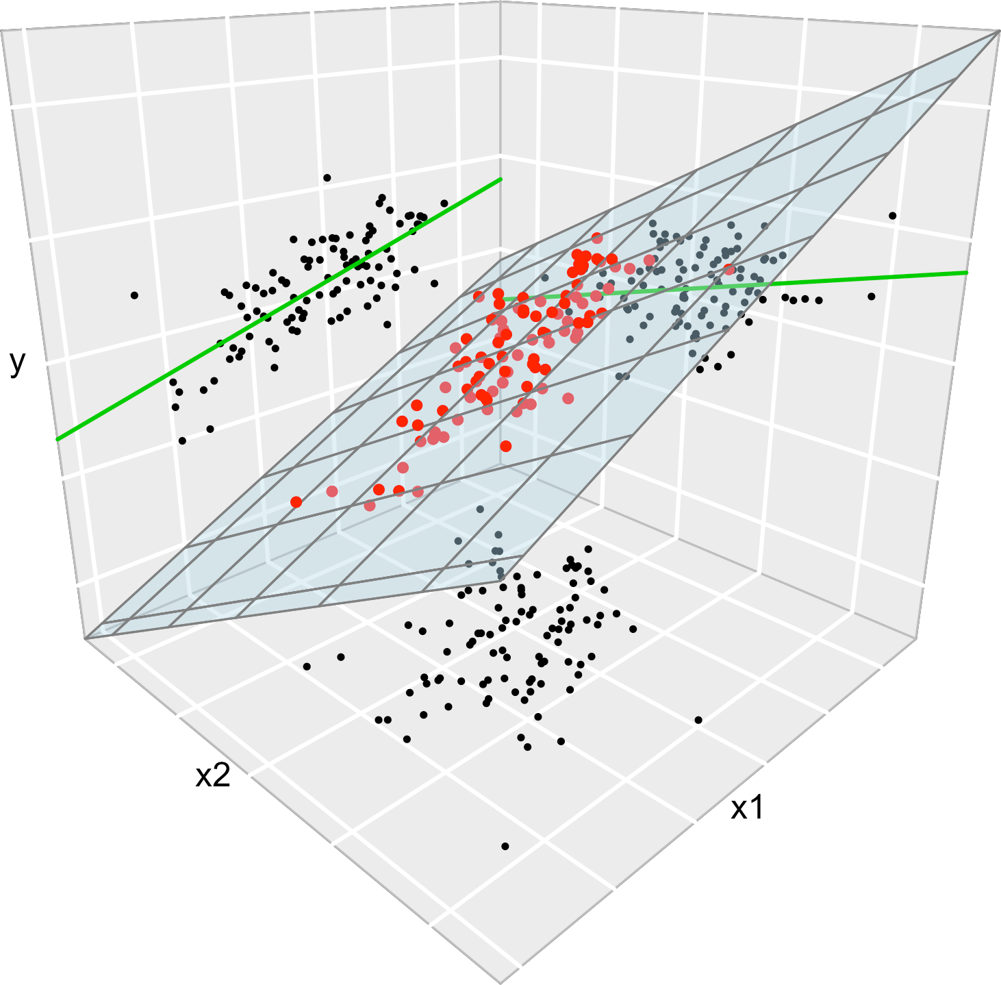
$The regression plane (blue) of $Y$ on $X_1$ and $X_2,$ and its relation with the regression lines (green lines) of $Y$ on $X_1$ (left) and $Y$ on $X_2$ (right). The red points represent the sample for $(X_1,X_2,Y)$ and the black points the subsamples for $(X_1,X_2)$ (bottom), $(X_1,Y)$ (left) and $(X_2,Y)$ (right). Note that the regression plane is not a direct extension of the marginal regression lines.$

Figure 3.1: The regression plane (blue) of $Y$ on $X_1$ and $X_2,$ and its relation with the regression lines (green lines) of $Y$ on $X_1$ (left) and $Y$ on $X_2$ (right). The red points represent the sample for $(X_1,X_2,Y)$ and the black points the subsamples for $(X_1,X_2)$ (bottom), $(X_1,Y)$ (left) and $(X_2,Y)$ (right). Note that the regression plane is not a direct extension of the marginal regression lines.

The estimation of $\beta_0,\beta_1,\ldots,\beta_p$ is done by minimizing the so-called Residual Sum of Squares (RSS). First we need to introduce some helpful matrix notation:

A sample of $(X_1,\ldots,X_p,Y)$ is denoted by $(X_{11},\ldots,X_{1p},Y_1),\allowbreak \ldots,(X_{n1},\ldots,X_{np},Y_n),$ where $X_{ij}$ denotes the $i$ -th observation of the $j$ -th predictor $X_j.$ We denote with $\mathbf{X}_i=(X_{i1},\ldots,X_{ip})$ to the $i$ -th observation of $(X_1,\ldots,X_p),$ so the sample simplifies to $(\mathbf{X}_{1},Y_1),\ldots,(\mathbf{X}_{n},Y_n).$
The design matrix contains all the information of the predictors and a column of ones

$\begin{align*} \mathbf{X}=\begin{pmatrix} 1 & X_{11} & \cdots & X_{1p}\\ \vdots & \vdots & \ddots & \vdots\\ 1 & X_{n1} & \cdots & X_{np} \end{pmatrix}_{n\times(p+1)}. \end{align*}$
The vector of responses $\mathbf{Y},$ the vector of coefficients $\boldsymbol\beta$ and the vector of errors are, respectively,

$\begin{align*} \mathbf{Y}=\begin{pmatrix} Y_1 \\ \vdots \\ Y_n \end{pmatrix}_{n\times 1},\quad\boldsymbol\beta=\begin{pmatrix} \beta_0 \\ \beta_1 \\ \vdots \\ \beta_p \end{pmatrix}_{(p+1)\times 1},\text{ and } \boldsymbol\varepsilon=\begin{pmatrix} \varepsilon_1 \\ \vdots \\ \varepsilon_n \end{pmatrix}_{n\times 1}. \end{align*}$

Thanks to the matrix notation, we can turn the sample version of the multiple linear model, namely

$\begin{align*} Y_i&=\beta_0 + \beta_1 X_{i1} + \cdots +\beta_p X_{ik} + \varepsilon_i,\quad i=1,\ldots,n, \end{align*}$

into something as compact as

$\begin{align*} \mathbf{Y}=\mathbf{X}\boldsymbol\beta+\boldsymbol\varepsilon. \end{align*}$

The RSS for the multiple linear regression is

$\begin{align} \text{RSS}(\boldsymbol\beta):=&\,\sum_{i=1}^n(Y_i-\beta_0-\beta_1X_{i1}-\cdots-\beta_pX_{ik})^2\nonumber\\ =&\,(\mathbf{Y}-\mathbf{X}\boldsymbol{\beta})'(\mathbf{Y}-\mathbf{X}\boldsymbol{\beta}).\tag{3.3} \end{align}$

The RSS aggregates the squared vertical distances from the data to a regression plane given by $\boldsymbol\beta.$ Note that the vertical distances are considered because we want to minimize the error in the prediction of $Y.$ Thus, the treatment of the variables is not symmetrical¹⁰; see Figure 3.2. The least squares estimators are the minimizers of the RSS:

$\begin{align*} \hat{\boldsymbol{\beta}}:=\arg\min_{\boldsymbol{\beta}\in\mathbb{R}^{p+1}} \text{RSS}(\boldsymbol{\beta}). \end{align*}$

Luckily, thanks to the matrix form of (3.3), it is simple to compute a closed-form expression for the least squares estimates:

$\begin{align} \hat{\boldsymbol{\beta}}=(\mathbf{X}'\mathbf{X})^{-1}\mathbf{X}'\mathbf{Y}.\tag{3.4} \end{align}$

Exercise 3.1 $\hat{\boldsymbol{\beta}}$ can be obtained differentiating (3.3). Prove it using that $\frac{\partial \mathbf{A}\mathbf{x}}{\partial \mathbf{x}}=\mathbf{A}$ and $\frac{\partial f(\mathbf{x})'g(\mathbf{x})}{\partial \mathbf{x}}=f(\mathbf{x})'\frac{\partial g(\mathbf{x})}{\partial \mathbf{x}}+g(\mathbf{x})'\frac{\partial f(\mathbf{x})}{\partial \mathbf{x}}$ for two vector-valued functions $f$ and $g.$

Figure 3.2: The least squares regression plane $y=\hat\beta_0+\hat\beta_1x_1+\hat\beta_2x_2$ and its dependence on the kind of squared distance considered. Application also available here.

Let’s check that indeed the coefficients given by R’s lm are the ones given by (3.4) in a toy linear model.

# Create the data employed in Figure 3.1

# Generates 50 points from a N(0, 1): predictors and error
set.seed(34567)
x1 <- rnorm(50)
x2 <- rnorm(50)
x3 <- x1 + rnorm(50, sd = 0.05) # Make variables dependent
eps <- rnorm(50)

# Responses
yLin <- -0.5 + 0.5 * x1 + 0.5 * x2 + eps
yQua <- -0.5 + x1^2 + 0.5 * x2 + eps
yExp <- -0.5 + 0.5 * exp(x2) + x3 + eps

# Data
dataAnimation <- data.frame(x1 = x1, x2 = x2, yLin = yLin,
                            yQua = yQua, yExp = yExp)

# Call lm
# lm employs formula = response ~ predictor1 + predictor2 + ...
# (names according to the data frame names) for denoting the regression
# to be done
mod <- lm(yLin ~ x1 + x2, data = dataAnimation)
summary(mod)
## 
## Call:
## lm(formula = yLin ~ x1 + x2, data = dataAnimation)
## 
## Residuals:
##      Min       1Q   Median       3Q      Max 
## -2.37003 -0.54305  0.06741  0.75612  1.63829 
## 
## Coefficients:
##             Estimate Std. Error t value Pr(>|t|)    
## (Intercept)  -0.5703     0.1302  -4.380 6.59e-05 ***
## x1            0.4833     0.1264   3.824 0.000386 ***
## x2            0.3215     0.1426   2.255 0.028831 *  
## ---
## Signif. codes:  0 '***' 0.001 '**' 0.01 '*' 0.05 '.' 0.1 ' ' 1
## 
## Residual standard error: 0.9132 on 47 degrees of freedom
## Multiple R-squared:  0.276,  Adjusted R-squared:  0.2452 
## F-statistic: 8.958 on 2 and 47 DF,  p-value: 0.0005057

# mod is a list with a lot of information
# str(mod) # Long output

# Coefficients
mod$coefficients
## (Intercept)          x1          x2 
##  -0.5702694   0.4832624   0.3214894

# Application of formula (3.4)

# Matrix X
X <- cbind(1, x1, x2)

# Vector Y
Y <- yLin

# Coefficients
beta <- solve(t(X) %*% X) %*% t(X) %*% Y
beta
##          [,1]
##    -0.5702694
## x1  0.4832624
## x2  0.3214894

Exercise 3.2 Compute $\boldsymbol{\beta}$ for the regressions yLin ~ x1 + x2, yQua ~ x1 + x2, and yExp ~ x2 + x3 using equation (3.4) and the function lm. Check that the fitted plane and the coefficient estimates are coherent.

Once we have the least squares estimates $\hat{\boldsymbol{\beta}},$ we can define the next two concepts:

The fitted values $\hat Y_1,\ldots,\hat Y_n,$ where

$\begin{align*} \hat Y_i:=\hat\beta_0+\hat\beta_1X_{i1}+\cdots+\hat\beta_pX_{ik},\quad i=1,\ldots,n. \end{align*}$

They are the vertical projections of $Y_1,\ldots,Y_n$ into the fitted line (see Figure 3.2). In a matrix form, inputting (3.3)

$\begin{align*} \hat{\mathbf{Y}}=\mathbf{X}\hat{\boldsymbol{\beta}}=\mathbf{X}(\mathbf{X}'\mathbf{X})^{-1}\mathbf{X}'\mathbf{Y}=\mathbf{H}\mathbf{Y}, \end{align*}$

where $\mathbf{H}:=\mathbf{X}(\mathbf{X}'\mathbf{X})^{-1}\mathbf{X}'$ is called the hat matrix because it “puts the hat into $\mathbf{Y}$ .” What it does is to project $\mathbf{Y}$ into the regression plane (see Figure 3.2).
The residuals (or estimated errors) $\hat \varepsilon_1,\ldots,\hat \varepsilon_n,$ where

$\begin{align*} \hat\varepsilon_i:=Y_i-\hat Y_i,\quad i=1,\ldots,n. \end{align*}$

They are the vertical distances between actual data and fitted data.

Model assumptions

Up to now, we have not made any probabilistic assumption on the data generation process. $\hat{\boldsymbol{\beta}}$ was derived from purely geometrical arguments, not probabilistic ones. However, some probabilistic assumptions are required for inferring the unknown population coefficients $\boldsymbol{\beta}$ from the sample $(\mathbf{X}_1, Y_1),\ldots,(\mathbf{X}_n, Y_n).$

The assumptions of the multiple linear model are:

Linearity: $\mathbb{E}[Y|X_1=x_1,\ldots,X_p=x_p]=\beta_0+\beta_1x_1+\cdots+\beta_px_p.$
Homoscedasticity: $\mathbb{V}\text{ar}[\varepsilon_i]=\sigma^2,$ with $\sigma^2$ constant for $i=1,\ldots,n.$
Normality: $\varepsilon_i\sim\mathcal{N}(0,\sigma^2)$ for $i=1,\ldots,n.$
Independence of the errors: $\varepsilon_1,\ldots,\varepsilon_n$ are independent (or uncorrelated, $\mathbb{E}[\varepsilon_i\varepsilon_j]=0,$ $i\neq j,$ since they are assumed to be normal).

A good one-line summary of the linear model is the following (independence is assumed)

$\begin{align} Y|(X_1=x_1,\ldots,X_p=x_p)\sim \mathcal{N}(\beta_0+\beta_1x_1+\cdots+\beta_px_p,\sigma^2).\tag{3.5} \end{align}$

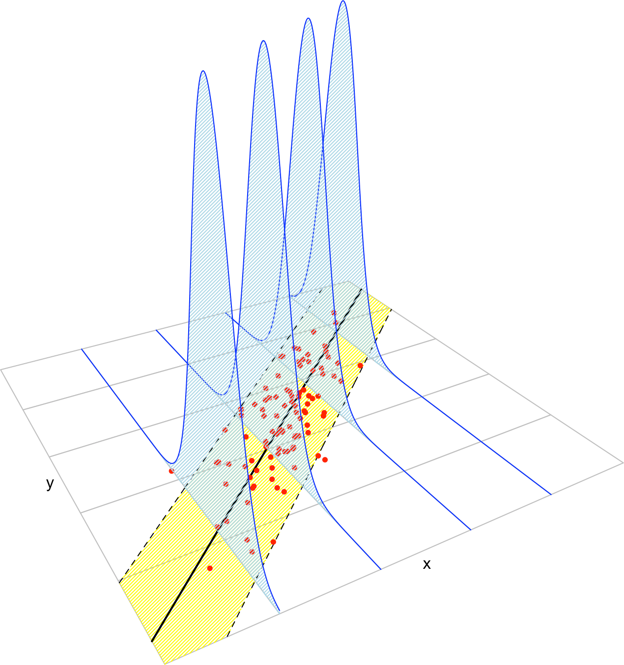
$The key concepts of the simple linear model. The blue densities denote the conditional density of $Y$ for each cut in the $X$ axis. The yellow band denotes where the $95\%$ of the data is, according to the model. The red points represent data following the model.$

Figure 3.3: The key concepts of the simple linear model. The blue densities denote the conditional density of $Y$ for each cut in the $X$ axis. The yellow band denotes where the $95\%$ of the data is, according to the model. The red points represent data following the model.

Inference on the parameters $\boldsymbol\beta$ and $\sigma$ can be done, conditionally¹¹ on $X_1,\ldots,X_n,$ from (3.5). We do not explore this further, referring the interested reader to these notes. Instead of that, we remark the connection between least squares estimation and the maximum likelihood estimator derived from (3.5).

First, note that (3.5) is the population version of the linear model (it is expressed in terms of the random variables, not in terms of their samples). The sample version that summarizes assumptions i–iv is

$\begin{align*} \mathbf{Y}|(\mathbf{X}_1,\ldots,\mathbf{X}_p)\sim \mathcal{N}_n(\mathbf{X}\boldsymbol{\beta},\sigma^2\mathbf{I}). \end{align*}$

Using this result, it is easy obtain the log-likelihood function of $Y_1,\ldots,Y_n$ conditionally¹² on $\mathbf{X}_1,\ldots,\mathbf{X}_n$ as

$\begin{align} \ell(\boldsymbol{\beta})=\log\phi_{\sigma^2\mathbf{I}}(\mathbf{Y}-\mathbf{X}\boldsymbol{\beta})=\sum_{i=1}^n\log\phi_{\sigma}(Y_i-(\mathbf{X}\boldsymbol{\beta})_i).\tag{3.6} \end{align}$

Finally, the next result justifies the consideration of the least squares estimate: it equals the maximum likelihood estimator derived under assumptions i–iv.

Theorem 3.1 Under assumptions i–iv, the maximum likelihood estimate of $\boldsymbol{\beta}$ is the least squares estimate (3.4):

$\begin{align*} \hat{\boldsymbol{\beta}}_\mathrm{ML}=\arg\max_{\boldsymbol{\beta}\in\mathbb{R}^{p+1}}\ell(\boldsymbol{\beta})=(\mathbf{X}'\mathbf{X})^{-1}\mathbf{X}\mathbf{Y}. \end{align*}$

Proof. Expanding the first equality at (3.6) gives ( $|\sigma^2\mathbf{I}|^{1/2}=\sigma^{n}$ )

$\begin{align*} \ell(\boldsymbol{\beta})=-\log((2\pi)^{n/2}\sigma^n)-\frac{1}{2\sigma^2}(\mathbf{Y}-\mathbf{X}\boldsymbol{\beta})'(\mathbf{Y}-\mathbf{X}\boldsymbol{\beta}). \end{align*}$

Optimizing $\ell$ does not require knowledge on $\sigma^2,$ since differentiating with respect to $\boldsymbol{\beta}$ and equating to zero gives (see Exercise 3.1) $\frac{1}{\sigma^2}(\mathbf{Y}-\mathbf{X}\boldsymbol{\beta})'\mathbf{X}=0.$ The result follows from that.

3.1.2 Logistic regression

Model formulation

When the response $Y$ can take only two values, codified for convenience as $1$ (success) and $0$ (failure), it is called a binary variable. A binary variable, known also as a Bernoulli variable, is a $\mathrm{B}(1, p).$ Recall that $\mathbb{E}[\mathrm{B}(1, p)]=\mathbb{P}[\mathrm{B}(1, p)=1]=p.$

If $Y$ is a binary variable and $X_1,\ldots,X_p$ are predictors associated to $Y,$ the purpose in logistic regression is to estimate

$\begin{align} p(x_1,\ldots,x_p):=&\,\mathbb{P}[Y=1|X_1=x_1,\ldots,X_p=x_p]\nonumber\\ =&\,\mathbb{E}[Y|X_1=x_1,\ldots,X_p=x_p],\tag{3.7} \end{align}$

this is, how the probability of $Y=1$ is changing according to particular values, denoted by $x_1,\ldots,x_p,$ of the predictors $X_1,\ldots,X_p.$ A tempting possibility is to consider a linear model for (3.7), $p(x_1,\ldots,x_p)=\beta_0+\beta_1x_1+\cdots+\beta_px_p.$ However, such a model will run into serious problems inevitably: negative probabilities and probabilities larger than one will arise.

A solution is to consider a function to encapsulate the value of $z=\beta_0+\beta_1x_1+\cdots+\beta_px_p,$ in $\mathbb{R},$ and map it back to $[0,1].$ There are several alternatives to do so, based on distribution functions $F:\mathbb{R}\longrightarrow[0,1]$ that deliver $y=F(z)\in[0,1].$ Different choices of $F$ give rise to different models, the most common being the logistic distribution function:

$\begin{align*} \mathrm{logistic}(z):=\frac{e^z}{1+e^z}=\frac{1}{1+e^{-z}}. \end{align*}$

Its inverse, $F^{-1}:[0,1]\longrightarrow\mathbb{R},$ known as the logit function, is

$\begin{align*} \mathrm{logit}(p):=\mathrm{logistic}^{-1}(p)=\log\frac{p}{1-p}. \end{align*}$

This is a link function, this is, a function that maps a given space (in this case $[0,1]$ ) into $\mathbb{R}.$ The term link function is employed in generalized linear models, which follow exactly the same philosophy of the logistic regression – mapping the domain of $Y$ to $\mathbb{R}$ in order to apply there a linear model. As said, different link functions are possible, but we will concentrate here exclusively on the logit as a link function.

The logistic model is defined as the following parametric form for (3.7):

$\begin{align} p(x_1,\ldots,x_p)&=\mathrm{logistic}(\beta_0+\beta_1x_1+\cdots+\beta_px_p)\nonumber\\ &=\frac{1}{1+e^{-(\beta_0+\beta_1x_1+\cdots+\beta_px_p)}}.\tag{3.8} \end{align}$

The linear form inside the exponent has a clear interpretation:

If $\beta_0+\beta_1x_1+\cdots+\beta_px_p=0,$ then $p(x_1,\ldots,x_p)=\frac{1}{2}$ ( $Y=1$ and $Y=0$ are equally likely).
If $\beta_0+\beta_1x_1+\cdots+\beta_px_p<0,$ then $p(x_1,\ldots,x_p)<\frac{1}{2}$ ( $Y=1$ less likely).
If $\beta_0+\beta_1x_1+\cdots+\beta_px_p>0,$ then $p(x_1,\ldots,x_p)>\frac{1}{2}$ ( $Y=1$ more likely).

To be more precise on the interpretation of the coefficients $\beta_0,\ldots,\beta_p$ we need to introduce the concept of odds. The odds is an equivalent way of expressing the distribution of probabilities in a binary variable. Since $\mathbb{P}[Y=1]=p$ and $\mathbb{P}[Y=0]=1-p,$ both the success and failure probabilities can be inferred from $p.$ Instead of using $p$ to characterize the distribution of $Y,$ we can use

$\begin{align} \mathrm{odds}(Y)=\frac{p}{1-p}=\frac{\mathbb{P}[Y=1]}{\mathbb{P}[Y=0]}.\tag{3.9} \end{align}$

The odds is the ratio between the probability of success and the probability of failure. It is extensively used in betting due to its better interpretability. For example, if a horse $Y$ has a probability $p=2/3$ of winning a race ( $Y=1$ ), then the odds of the horse is

$\begin{align*} \text{odds}=\frac{p}{1-p}=\frac{2/3}{1/3}=2. \end{align*}$

This means that the horse has a probability of winning that is twice larger than the probability of losing. This is sometimes written as a $2:1$ or $2 \times 1$ (spelled “two-to-one”). Conversely, if the odds of $Y$ is given, we can easily know what is the probability of success $p,$ using the inverse of (3.9):

$\begin{align*} p=\mathbb{P}[Y=1]=\frac{\text{odds}(Y)}{1+\text{odds}(Y)}. \end{align*}$

For example, if the odds of the horse were $5,$ that would correspond to a probability of winning $p=5/6.$

Remark. Recall that the odds is a number in $[0,+\infty].$ The $0$ and $+\infty$ values are attained for $p=0$ and $p=1,$ respectively. The log-odds (or logit) is a number in $[-\infty,+\infty].$

We can rewrite (3.8) in terms of the odds (3.9). If we do so, we have:

$\begin{align*} \mathrm{odds}(Y|&X_1=x_1,\ldots,X_p=x_p)\\ &=\frac{p(x_1,\ldots,x_p)}{1-p(x_1,\ldots,x_p)}\\ &=e^{\beta_0+\beta_1x_1+\cdots+\beta_px_p}\\ &=e^{\beta_0}e^{\beta_1x_1}\ldots e^{\beta_px_p}. \end{align*}$

This provides the following interpretation of the coefficients:

$e^{\beta_0}$ : is the odds of $Y=1$ when $X_1=\ldots=X_p=0.$
$e^{\beta_j},$ $1\leq j\leq k$ : is the multiplicative increment of the odds for an increment of one unit in $X_j=x_j,$ provided that the remaining variables do not change. If the increment in $X_j$ is of $r$ units, then the multiplicative increment in the odds is $(e^{\beta_j})^r.$

Model assumptions and estimation

Some probabilistic assumptions are required for performing inference on the model parameters $\boldsymbol\beta$ from the sample $(\mathbf{X}_1, Y_1),\ldots,(\mathbf{X}_n, Y_n).$ These assumptions are somehow simpler than the ones for linear regression.

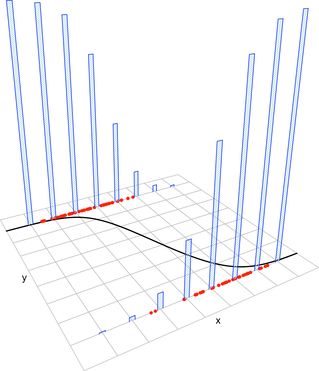
$The key concepts of the logistic model. The blue bars represent the conditional distribution of probability of $Y$ for each cut in the $X$ axis. The red points represent data following the model.$

Figure 3.4: The key concepts of the logistic model. The blue bars represent the conditional distribution of probability of $Y$ for each cut in the $X$ axis. The red points represent data following the model.

The assumptions of the logistic model are the following:

Linearity in the logit¹³: $\mathrm{logit}(p(\mathbf{x}))=\log\frac{ p(\mathbf{x})}{1-p(\mathbf{x})}=\beta_0+\beta_1x_1+\cdots+\beta_px_p.$
Binariness: $Y_1,\ldots,Y_n$ are binary variables.
Independence: $Y_1,\ldots,Y_n$ are independent.

A good one-line summary of the logistic model is the following (independence is assumed)

$\begin{align*} Y|(X_1=x_1,\ldots,X_p=x_p)&\sim\mathrm{Ber}\left(\mathrm{logistic}(\beta_0+\beta_1x_1+\cdots+\beta_px_p)\right)\\ &=\mathrm{Ber}\left(\frac{1}{1+e^{-(\beta_0+\beta_1x_1+\cdots+\beta_px_p)}}\right). \end{align*}$

Since $Y_i\sim \mathrm{Ber}(p(\mathbf{X}_i)),$ $i=1,\ldots,n,$ the log-likelihood of $\boldsymbol{\beta}$ is

$\begin{align} \ell(\boldsymbol{\beta})=&\,\sum_{i=1}^n\log\left(p(\mathbf{X}_i)^{Y_i}(1-p(\mathbf{X}_i))^{1-Y_i}\right)\nonumber\\ =&\,\sum_{i=1}^n\left\{Y_i\log(p(\mathbf{X}_i))+(1-Y_i)\log(1-p(\mathbf{X}_i))\right\}.\tag{3.10} \end{align}$

Unfortunately, due to the non-linearity of the optimization problem there are no explicit expressions for $\hat{\boldsymbol{\beta}}.$ These have to be obtained numerically by means of an iterative procedure, which may run into problems in low sample situations with perfect classification. Unlike in the linear model, inference is not exact from the assumptions, but approximate in terms of maximum likelihood theory. We do not explore this further and refer the interested reader to these notes.

Figure 3.5: The logistic regression fit and its dependence on $\beta_0$ (horizontal displacement) and $\beta_1$ (steepness of the curve). Recall the effect of the sign of $\beta_1$ in the curve: if positive, the logistic curve has an ‘s’ form; if negative, the form is a reflected ‘s.’ Application also available here.

Figure 3.5 shows how the log-likelihood changes with respect to the values for $(\beta_0,\beta_1)$ in three data patterns.

The data of the illustration has been generated with the following code:

# Create the data employed in Figure 3.4

# Data
set.seed(34567)
x <- rnorm(50, sd = 1.5)
y1 <- -0.5 + 3 * x
y2 <- 0.5 - 2 * x
y3 <- -2 + 5 * x
y1 <- rbinom(50, size = 1, prob = 1 / (1 + exp(-y1)))
y2 <- rbinom(50, size = 1, prob = 1 / (1 + exp(-y2)))
y3 <- rbinom(50, size = 1, prob = 1 / (1 + exp(-y3)))

# Data
dataMle <- data.frame(x = x, y1 = y1, y2 = y2, y3 = y3)

Let’s check that indeed the coefficients given by R’s glm are the ones that maximize the likelihood of the animation of Figure 3.5. We do so for y ~ x1.

# Call glm
# glm employs formula = response ~ predictor1 + predictor2 + ...
# (names according to the data frame names) for denoting the regression
# to be done. We need to specify family = "binomial" to make a
# logistic regression
mod <- glm(y1 ~ x, family = "binomial", data = dataMle)
summary(mod)
## 
## Call:
## glm(formula = y1 ~ x, family = "binomial", data = dataMle)
## 
## Deviance Residuals: 
##      Min        1Q    Median        3Q       Max  
## -2.47853  -0.40139   0.02097   0.38880   2.12362  
## 
## Coefficients:
##             Estimate Std. Error z value Pr(>|z|)    
## (Intercept)  -0.1692     0.4725  -0.358 0.720274    
## x             2.4282     0.6599   3.679 0.000234 ***
## ---
## Signif. codes:  0 '***' 0.001 '**' 0.01 '*' 0.05 '.' 0.1 ' ' 1
## 
## (Dispersion parameter for binomial family taken to be 1)
## 
##     Null deviance: 69.315  on 49  degrees of freedom
## Residual deviance: 29.588  on 48  degrees of freedom
## AIC: 33.588
## 
## Number of Fisher Scoring iterations: 6

# mod is a list with a lot of information
# str(mod) # Long output

# Coefficients
mod$coefficients
## (Intercept)           x 
##  -0.1691947   2.4281626

# Plot the fitted regression curve
xGrid <- seq(-5, 5, l = 200)
yGrid <- 1 / (1 + exp(-(mod$coefficients[1] + mod$coefficients[2] * xGrid)))
plot(xGrid, yGrid, type = "l", col = 2, xlab = "x", ylab = "y")
points(x, y1)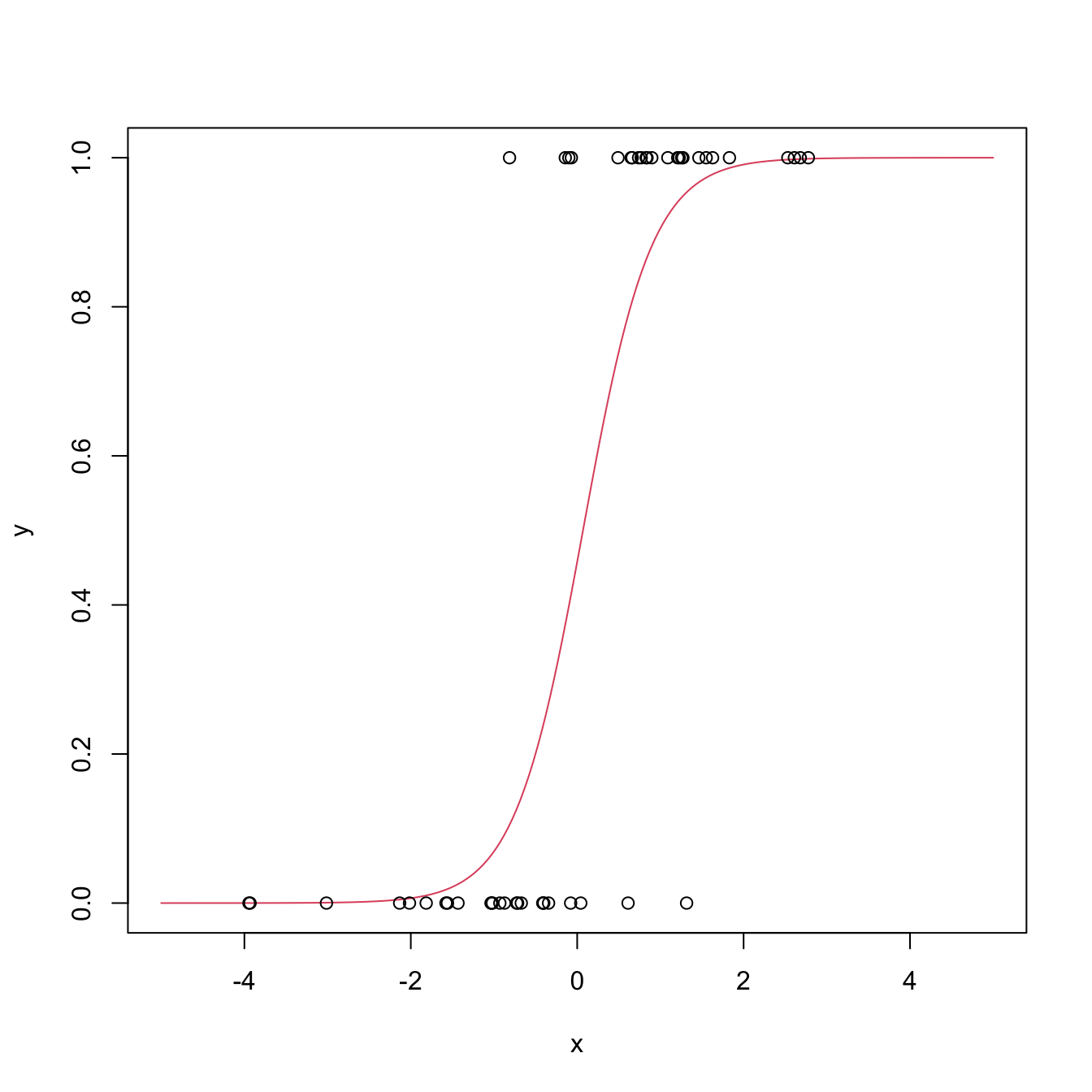

Exercise 3.3 For the regressions y ~ x2 and y ~ x3, do the following:

Check that $\boldsymbol{\beta}$ is indeed maximizing the likelihood as compared with Figure 3.5.
Plot the fitted logistic curve and compare it with the one in Figure 3.5.

Not to confuse with a sample!↩︎
If that was the case, we would consider perpendicular distances, which yield to Principal Component Analysis (PCA).↩︎
We assume that the randomness is on the response only.↩︎
We assume that the randomness is on the response only.↩︎
An equivalent way of stating this assumption is $p(\mathbf{x})=\mathrm{logistic}(\beta_0+\beta_1x_1+\cdots+\beta_px_p).$ ↩︎