3.2 Kernel regression estimation
3.2.1 Nadaraya–Watson estimator
Our objective is to estimate the regression function \(m\) nonparametrically. Due to its definition, we can rewrite it as follows:
\[\begin{align*} m(x)=&\,\mathbb{E}[Y\vert X=x]\nonumber\\ =&\,\int y f_{Y\vert X=x}(y)\,\mathrm{d}y\nonumber\\ =&\,\frac{\int y f(x,y)\,\mathrm{d}y}{f_X(x)}. \end{align*}\]
This expression shows an interesting point: the regression function can be computed from the joint density \(f\) and the marginal \(f_X.\) Therefore, given a sample \((X_1,Y_1),\ldots,(X_n,Y_n),\) an estimate of \(m\) follows by replacing the previous densities by their kdes. To that aim, recall that in Exercise 2.15 we defined a multivariate extension of the kde based on product kernels. For the two dimensional case, the kde with equal bandwidths \(\mathbf{h}=(h,h)\) is
\[\begin{align} \hat f(x,y;h)=\frac{1}{n}\sum_{i=1}^nK_{h}(x_1-X_{i})K_{h}(y-Y_{i}).\tag{3.11} \end{align}\]
Using (3.11),
\[\begin{align*} m(x)\approx&\,\frac{\int y \hat f(x,y;h)\,\mathrm{d}y}{\hat f_X(x;h)}\\ =&\,\frac{\int y \hat f(x,y;h)\,\mathrm{d}y}{\hat f_X(x;h)}\\ =&\,\frac{\int y \frac{1}{n}\sum_{i=1}^nK_h(x-X_i)K_h(y-Y_i)\,\mathrm{d}y}{\frac{1}{n}\sum_{i=1}^nK_h(x-X_i)}\\ =&\,\frac{\frac{1}{n}\sum_{i=1}^nK_h(x-X_i)\int y K_h(y-Y_i)\,\mathrm{d}y}{\frac{1}{n}\sum_{i=1}^nK_h(x-X_i)}\\ =&\,\frac{\frac{1}{n}\sum_{i=1}^nK_h(x-X_i)Y_i}{\frac{1}{n}\sum_{i=1}^nK_h(x-X_i)}. \end{align*}\]
This yields the so-called Nadaraya–Watson14 estimate:
\[\begin{align} \hat m(x;0,h):=\frac{1}{n}\sum_{i=1}^n\frac{K_h(x-X_i)}{\frac{1}{n}\sum_{i=1}^nK_h(x-X_i)}Y_i=\sum_{i=1}^nW^0_{i}(x)Y_i, \tag{3.12} \end{align}\]
where \(W^0_{i}(x):=\frac{K_h(x-X_i)}{\sum_{i=1}^nK_h(x-X_i)}.\) This estimate can be seen as a weighted average of \(Y_1,\ldots,Y_n\) by means of the set of weights \(\{W_{n,i}(x)\}_{i=1}^n\) (check that they add to one). The set of weights depends on the evaluation point \(x.\) That means that the Nadaraya–Watson estimator is a local mean of \(Y_1,\ldots,Y_n\) around \(X=x\) (see Figure 3.6).
Let’s implement the Nadaraya–Watson estimate to get a feeling of how it works in practice.
# Nadaraya-Watson
mNW <- function(x, X, Y, h, K = dnorm) {

  # Arguments
  # x: evaluation points
  # X: vector (size n) with the predictors
  # Y: vector (size n) with the response variable
  # h: bandwidth
  # K: kernel

  # Matrix of size n x length(x)
  Kx <- sapply(X, function(Xi) K((x - Xi) / h) / h)

  # Weights
  W <- Kx / rowSums(Kx) # Column recycling!

  # Means at x ("drop" to drop the matrix attributes)
  drop(W %*% Y)

}

# Generate some data to test the implementation
set.seed(12345)
n <- 100
eps <- rnorm(n, sd = 2)
m <- function(x) x^2 * cos(x)
X <- rnorm(n, sd = 2)
Y <- m(X) + eps
xGrid <- seq(-10, 10, l = 500)

# Bandwidth
h <- 0.5

# Plot data
plot(X, Y)
rug(X, side = 1); rug(Y, side = 2)
lines(xGrid, m(xGrid), col = 1)
lines(xGrid, mNW(x = xGrid, X = X, Y = Y, h = h), col = 2)
legend("topright", legend = c("True regression", "Nadaraya-Watson"),
       lwd = 2, col = 1:2)
Exercise 3.4 Implement your own version of the Nadaraya–Watson estimator in R and compare it with mNW. You may focus only on the normal kernel and reduce the accuracy of the final computation up to 1e-7 to achieve better efficiency. Are you able to improve the speed of mNW? Use system.time or the microbenchmark package to measure the running times for a sample size of \(n=10000.\)
Winner-takes-all bonus: the significative fastest version of the Nadaraya–Watson estimator (under the above conditions) will get a bonus of 0.5 points.
The code below illustrates the effect of varying \(h\) for the Nadaraya–Watson estimator using manipulate.
# Simple plot of N-W for varying h's
manipulate({

  # Plot data
  plot(X, Y)
  rug(X, side = 1); rug(Y, side = 2)
  lines(xGrid, m(xGrid), col = 1)
  lines(xGrid, mNW(x = xGrid, X = X, Y = Y, h = h), col = 2)
  legend("topright", legend = c("True regression", "Nadaraya-Watson"),
         lwd = 2, col = 1:2)

}, h = slider(min = 0.01, max = 2, initial = 0.5, step = 0.01))
3.2.2 Local polynomial regression
Nadaraya–Watson can be seen as a particular case of a local polynomial fit, specifically, the one corresponding to a local constant fit. The motivation for the local polynomial fit comes from attempting to the minimize the RSS
\[\begin{align} \sum_{i=1}^n(Y_i-m(X_i))^2.\tag{3.13} \end{align}\]
This is not achievable directly, since no knowledge on \(m\) is available. However, by a \(p\)-th order Taylor expression it is possible to obtain that, for \(x\) close to \(X_i,\)
\[\begin{align} m(X_i)\approx&\, m(x)+m'(x)(X_i-x)+\frac{m''(x)}{2}(X_i-x)^2\nonumber\\ &+\cdots+\frac{m^{(p)}(x)}{p!}(X_i-x)^p.\tag{3.14} \end{align}\]
Replacing (3.14) in (3.13), we have that
\[\begin{align} \sum_{i=1}^n\left(Y_i-\sum_{j=0}^p\frac{m^{(j)}(x)}{j!}(X_i-x)^j\right)^2.\tag{3.15} \end{align}\]
This expression is still not workable: it depends on \(m^{(j)}(x),\) \(j=0,\ldots,p,\) which of course are unknown! The great idea is to set \(\beta_j:=\frac{m^{(j)}(x)}{j!}\) and turn (3.15) into a linear regression problem where the unknown parameters are \(\boldsymbol{\beta}=(\beta_0,\beta_1,\ldots,\beta_p)'\):
\[\begin{align} \sum_{i=1}^n\left(Y_i-\sum_{j=0}^p\beta_j(X_i-x)^j\right)^2.\tag{3.16} \end{align}\]
While doing so, an estimate of \(\boldsymbol{\beta}\) automatically will yield estimates for \(m^{(j)}(x),\) \(j=0,\ldots,p,\) and we know how to obtain \(\hat{\boldsymbol{\beta}}\) by minimizing (3.16). The final touch is to make the contributions of \(X_i\) dependent on the distance to \(x\) by weighting with kernels:
\[\begin{align} \hat{\boldsymbol{\beta}}:=\arg\min_{\boldsymbol{\beta}\in\mathbb{R}^{p+1}}\sum_{i=1}^n\left(Y_i-\sum_{j=0}^p\beta_j(X_i-x)^j\right)^2K_h(x-X_i).\tag{3.17} \end{align}\]
Denoting
\[\begin{align*} \mathbf{X}:=\begin{pmatrix} 1 & X_1-x & \cdots & (X_1-x)^p\\ \vdots & \vdots & \ddots & \vdots\\ 1 & X_n-x & \cdots & (X_n-x)^p\\ \end{pmatrix}_{n\times(p+1)} \end{align*}\]
and
\[\begin{align*} \mathbf{W}:=\mathrm{diag}(K_h(X_1-x),\ldots, K_h(X_n-x)),\quad \mathbf{Y}:=\begin{pmatrix} Y_1\\ \vdots\\ Y_n \end{pmatrix}_{n\times 1}, \end{align*}\]
we can re-express (3.17) into a weighted least squares problem whose exact solution is
\[\begin{align} \hat{\boldsymbol{\beta}}&=\arg\min_{\boldsymbol{\beta}\in\mathbb{R}^{p+1}} (\mathbf{Y}-\mathbf{X}\boldsymbol{\beta})'\mathbf{W}(\mathbf{Y}-\mathbf{X}\boldsymbol{\beta})\\ &=(\mathbf{X}'\mathbf{W}\mathbf{X})^{-1}\mathbf{X}'\mathbf{W}\mathbf{Y}.\tag{3.18} \end{align}\]
The estimate for \(m(x)\) is then computed as
\[\begin{align*} \hat m(x;p,h):&=\hat\beta_0\\ &=\mathbf{e}_1'(\mathbf{X}'\mathbf{W}\mathbf{X})^{-1}\mathbf{X}'\mathbf{W}\mathbf{Y}\\ &=\sum_{i=1}^nW^p_{i}(x)Y_i, \end{align*}\]
where \(W^p_{i}(x):=\mathbf{e}_1'(\mathbf{X}'\mathbf{W}\mathbf{X})^{-1}\mathbf{X}'\mathbf{W}\mathbf{e}_i\) and \(\mathbf{e}_i\) is the \(i\)-th canonical vector. Just as the Nadaraya–Watson, the local polynomial estimator is a linear combination of the responses. Two cases deserve special attention:
\(p=0\) is the local constant estimator or the Nadaraya–Watson estimator (Exercise 3.6). In this situation, the estimator has explicit weights, as we saw before:
\[\begin{align*} W_i^0(x)=\frac{K_h(x-X_i)}{\sum_{j=1}^nK_h(x-X_j)}. \end{align*}\]
\(p=1\) is the local linear estimator, which has weights equal to (Exercise 3.9):
\[\begin{align} W_i^1(x)=\frac{1}{n}\frac{\hat s_2(x;h)-\hat s_1(x;h)(X_i-x)}{\hat s_2(x;h)\hat s_0(x;h)-\hat s_1(x;h)^2}K_h(x-X_i),\tag{3.19} \end{align}\]
where \(\hat s_r(x;h):=\frac{1}{n}\sum_{i=1}^n(X_i-x)^rK_h(x-X_i).\)
Figure 3.6 illustrates the construction of the local polynomial estimator (up to cubic degree) and shows how \(\hat\beta_0=\hat m(x;p,h),\) the intercept of the local fit, estimates \(m\) at \(x.\)
Figure 3.6: Construction of the local polynomial estimator. The animation shows how local polynomial fits in a neighborhood of \(x\) are combined to provide an estimate of the regression function, which depends on the polynomial degree, bandwidth, and kernel (gray density at the bottom). The data points are shaded according to their weights for the local fit at \(x.\) Application also available here.
KernSmooth’s locpoly implements the local polynomial estimator. Below are some examples of its usage.
# Generate some data to test the implementation
set.seed(123456)
n <- 100
eps <- rnorm(n, sd = 2)
m <- function(x) x^3 * sin(x)
X <- rnorm(n, sd = 1.5)
Y <- m(X) + eps
xGrid <- seq(-10, 10, l = 500)

# Bandwidth
h <- 0.25
lp0 <- locpoly(x = X, y = Y, bandwidth = h, degree = 0, range.x = c(-10, 10),
               gridsize = 500)
lp1 <- locpoly(x = X, y = Y, bandwidth = h, degree = 1, range.x = c(-10, 10),
               gridsize = 500)

# Plot data
plot(X, Y)
rug(X, side = 1); rug(Y, side = 2)
lines(xGrid, m(xGrid), col = 1)
lines(lp0$x, lp0$y, col = 2)
lines(lp1$x, lp1$y, col = 3)
legend("bottom", legend = c("True regression", "Local constant",
                         "Local linear"),
       lwd = 2, col = 1:3)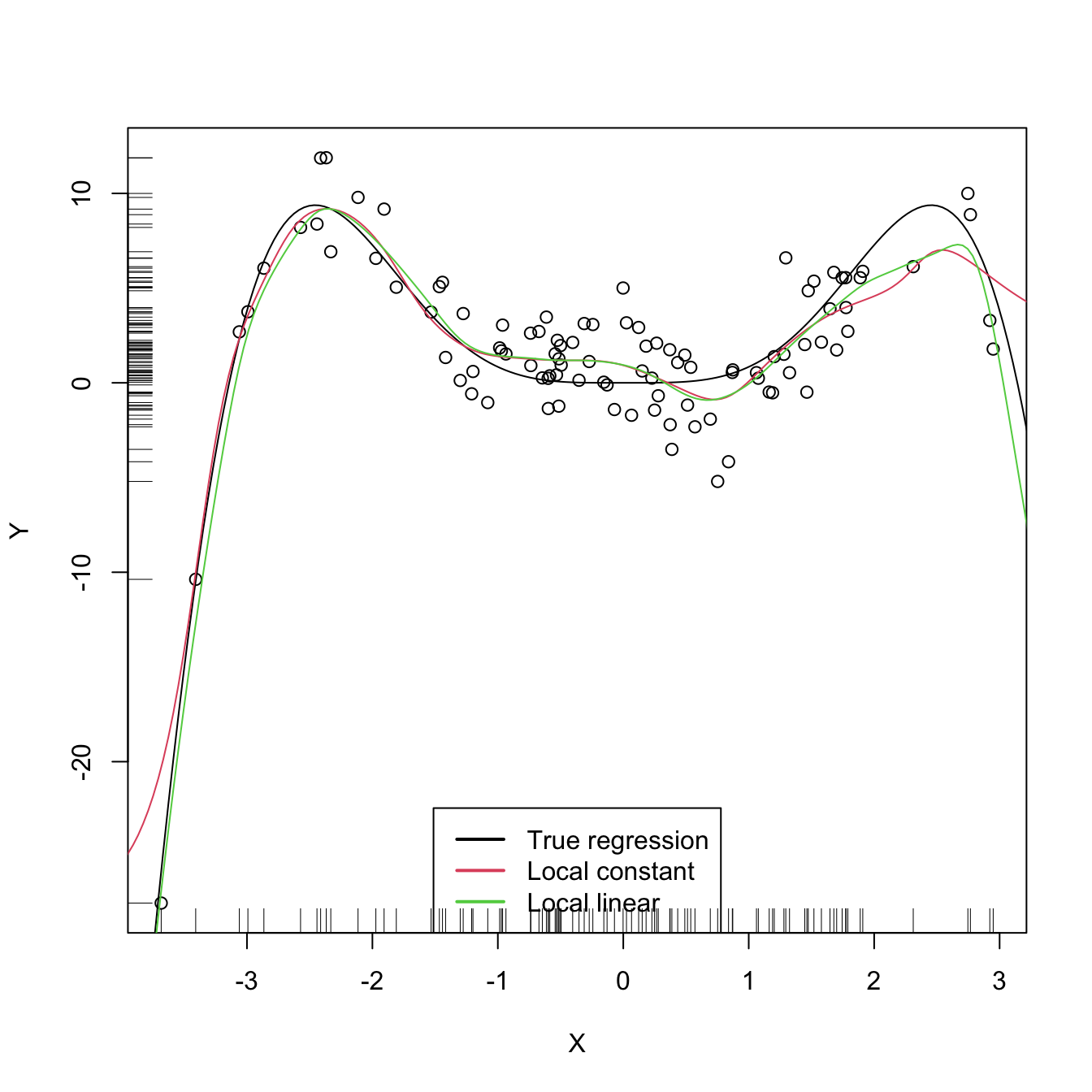
# Simple plot of local polynomials for varying h's
manipulate({

  # Plot data
  lpp <- locpoly(x = X, y = Y, bandwidth = h, degree = p, range.x = c(-10, 10),
                 gridsize = 500)
  plot(X, Y)
  rug(X, side = 1); rug(Y, side = 2)
  lines(xGrid, m(xGrid), col = 1)
  lines(lpp$x, lpp$y, col = p + 2)
  legend("bottom", legend = c("True regression", "Local polynomial fit"),
         lwd = 2, col = c(1, p + 2))

}, h = slider(min = 0.01, max = 2, initial = 0.5, step = 0.01),
p = slider(min = 0, max = 4, initial = 0, step = 1))