2.1 Histograms

2.1.1 Histogram

The simplest method to estimate a density $f$ from an iid sample $X_1,\ldots,X_n$ is the histogram. From an analytical point of view, the idea is to aggregate the data in intervals of the form $[x_0,x_0+h)$ and then use their relative frequency to approximate the density at $x\in[x_0,x_0+h),$ $f(x),$ by the estimate of

$\begin{align*} f(x_0)&=F'(x_0)\\ &=\lim_{h\to0^+}\frac{F(x_0+h)-F(x_0)}{h}\\ &=\lim_{h\to0^+}\frac{\mathbb{P}[x_0<X< x_0+h]}{h}. \end{align*}$

More precisely, given an origin $t_0$ and a bandwidth $h>0,$ the histogram builds a piecewise constant function in the intervals $\{B_k:=[t_{k},t_{k+1}):t_k=t_0+hk,k\in\mathbb{Z}\}$ by counting the number of sample points inside each of them. These constant-length intervals are also denoted bins. The fact that they are of constant length $h$ is important, since it allows to standardize by $h$ in order to have relative frequencies per length. The histogram at a point $x$ is defined as

$\begin{align} \hat f_\mathrm{H}(x;t_0,h):=\frac{1}{nh}\sum_{i=1}^n1_{\{X_i\in B_k:x\in B_k\}}. \tag{2.1} \end{align}$

Equivalently, if we denote the number of points in $B_k$ as $v_k,$ then the histogram is $\hat f_\mathrm{H}(x;t_0,h)=\frac{v_k}{nh}$ if $x\in B_k$ for a $k\in\mathbb{Z}.$

The analysis of $\hat f_\mathrm{H}(x;t_0,h)$ as a random variable is simple, once it is recognized that the bin counts $v_k$ are distributed as $\mathrm{B}(n,p_k),$ with $p_k=\mathbb{P}[X\in B_k]=\int_{B_k} f(t)\,\mathrm{d}t$ ⁴. If $f$ is continuous, then by the mean value theorem, $p_k=hf(\xi_{k,h})$ for a $\xi_{k,h}\in(t_k,t_{k+1}).$ Assume that $k\in\mathbb{Z}$ is such that $x\in B_k=[t_k,t_{k+1}).$ Therefore:

$\begin{align*} \mathbb{E}[\hat f_\mathrm{H}(x;t_0,h)]&=\frac{np_k}{nh}=f(\xi_{k,h}),\\ \mathbb{V}\mathrm{ar}[\hat f_\mathrm{H}(x;t_0,h)]&=\frac{np_k(1-p_k)}{n^2h^2}=\frac{f(\xi_{k,h})(1-hf(\xi_{k,h}))}{nh}. \end{align*}$

The above results show interesting insights:

If $h\to0,$ then $\xi_{h,k}\to x,$ resulting in $f(\xi_{k,h})\to f(x),$ and thus (2.1) becomes an asymptotically unbiased estimator of $f(x).$
But if $h\to0,$ the variance increases. For decreasing the variance, $nh\to\infty$ is required.
The variance is directly dependent on $f(x)(1-hf(x))\approx f(x),$ hence there is more variability at regions with high density.

A more detailed analysis of the histogram can be seen in Section 3.2.2 of Scott (2015). We skip it here since the detailed asymptotic analysis for the more general kernel density estimator is given in Section 2.2.

The implementation of histograms is very simple in R. As an example, we consider the old-but-gold dataset faithful. This dataset contains the duration of the eruption and the waiting time between eruptions for the Old Faithful geyser in Yellowstone National Park (USA).

# The faithful dataset is included in R
head(faithful)
##   eruptions waiting
## 1     3.600      79
## 2     1.800      54
## 3     3.333      74
## 4     2.283      62
## 5     4.533      85
## 6     2.883      55

# Duration of eruption
faithE <- faithful$eruptions

# Default histogram: automatically chosen bins and absolute frequencies!
histo <- hist(faithE)


# List that contains several objects
str(histo)
## List of 6
##  $ breaks  : num [1:9] 1.5 2 2.5 3 3.5 4 4.5 5 5.5
##  $ counts  : int [1:8] 55 37 5 9 34 75 54 3
##  $ density : num [1:8] 0.4044 0.2721 0.0368 0.0662 0.25 ...
##  $ mids    : num [1:8] 1.75 2.25 2.75 3.25 3.75 4.25 4.75 5.25
##  $ xname   : chr "faithE"
##  $ equidist: logi TRUE
##  - attr(*, "class")= chr "histogram"

# With relative frequencies
hist(faithE, probability = TRUE)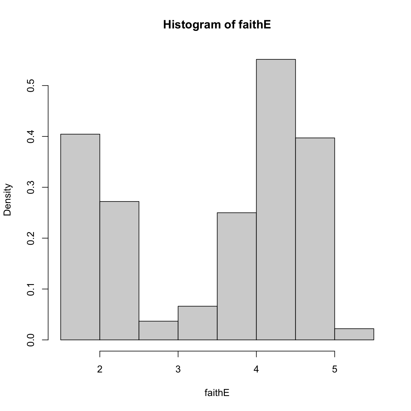


# Choosing the breaks
# t0 = min(faithE), h = 0.25
Bk <- seq(min(faithE), max(faithE), by = 0.25)
hist(faithE, probability = TRUE, breaks = Bk)
rug(faithE) # Plotting the sample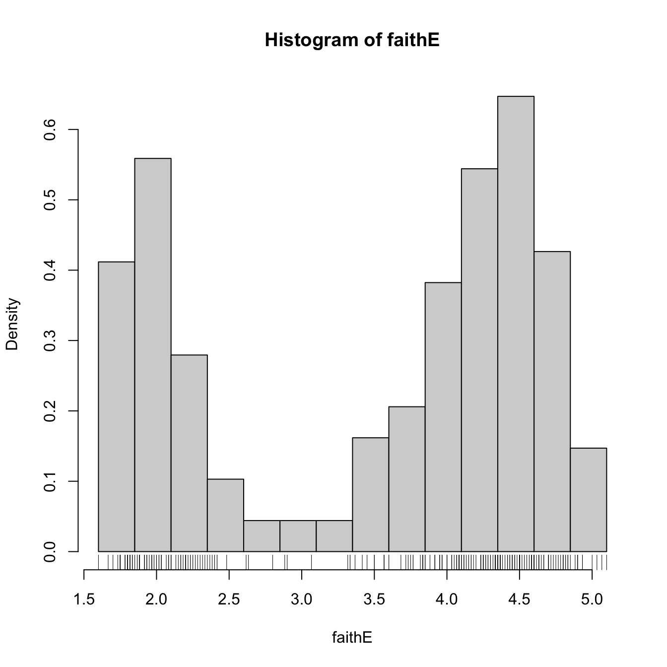

The shape of the histogram depends on:

$t_0,$ since the separation between bins happens at $t_0k,$ $k\in\mathbb{Z};$
$h,$ which controls the bin size and the effective number of bins for aggregating the sample.

We focus first on exploring the dependence on $t_0,$ as it serves for motivating the next density estimator.

# Uniform sample
set.seed(1234567)
u <- runif(n = 100)

# t0 = 0, h = 0.2
Bk1 <- seq(0, 1, by = 0.2)

# t0 = -0.1, h = 0.2
Bk2 <- seq(-0.1, 1.1, by = 0.2)

# Comparison
hist(u, probability = TRUE, breaks = Bk1, ylim = c(0, 1.5),
     main = "t0 = 0, h = 0.2")
rug(u)
abline(h = 1, col = 2)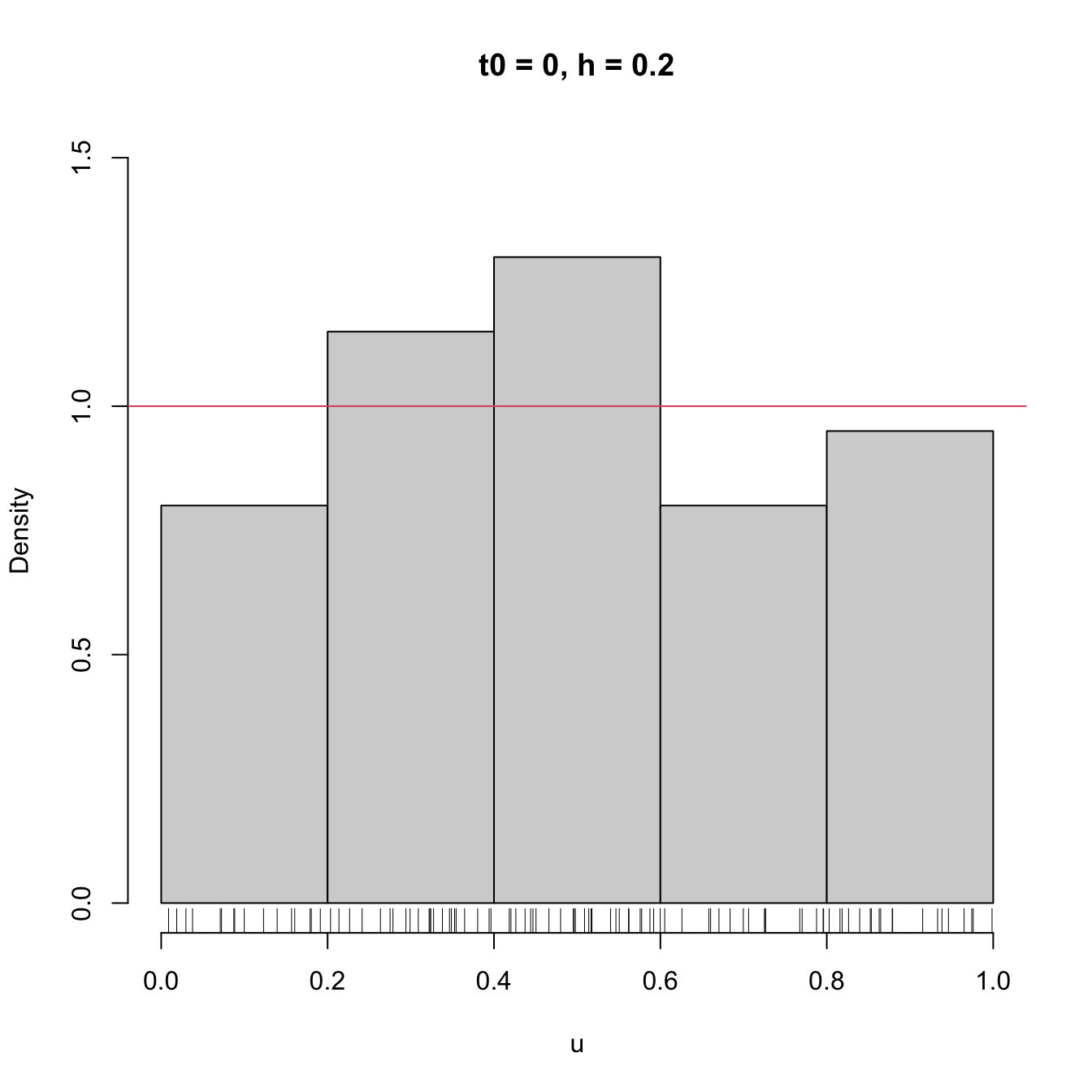

hist(u, probability = TRUE, breaks = Bk2, ylim = c(0, 1.5),
     main = "t0 = -0.1, h = 0.2")
rug(u)
abline(h = 1, col = 2)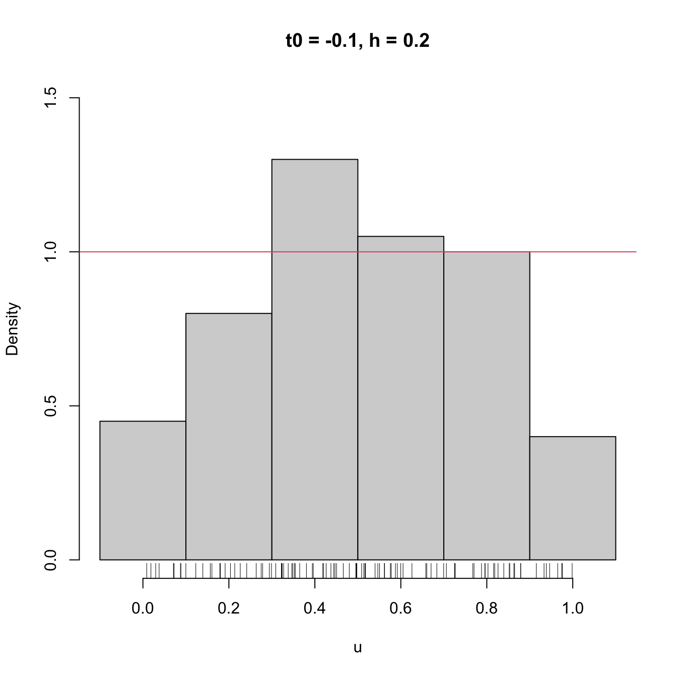

High dependence on $t_0$ also happens when estimating densities that are not compactly supported. The next snippet of code points towards it.

# Sample 100 points from a N(0, 1) and 50 from a N(3, 0.25)
set.seed(1234567)
samp <- c(rnorm(n = 100, mean = 0, sd = 1),
          rnorm(n = 50, mean = 3.25, sd = sqrt(0.5)))

# min and max for choosing Bk1 and Bk2
range(samp)
## [1] -2.107233  4.679118

# Comparison
Bk1 <- seq(-2.5, 5, by = 0.5)
Bk2 <- seq(-2.25, 5.25, by = 0.5)
hist(samp, probability = TRUE, breaks = Bk1, ylim = c(0, 0.5),
     main = "t0 = -2.5, h = 0.5")
rug(samp)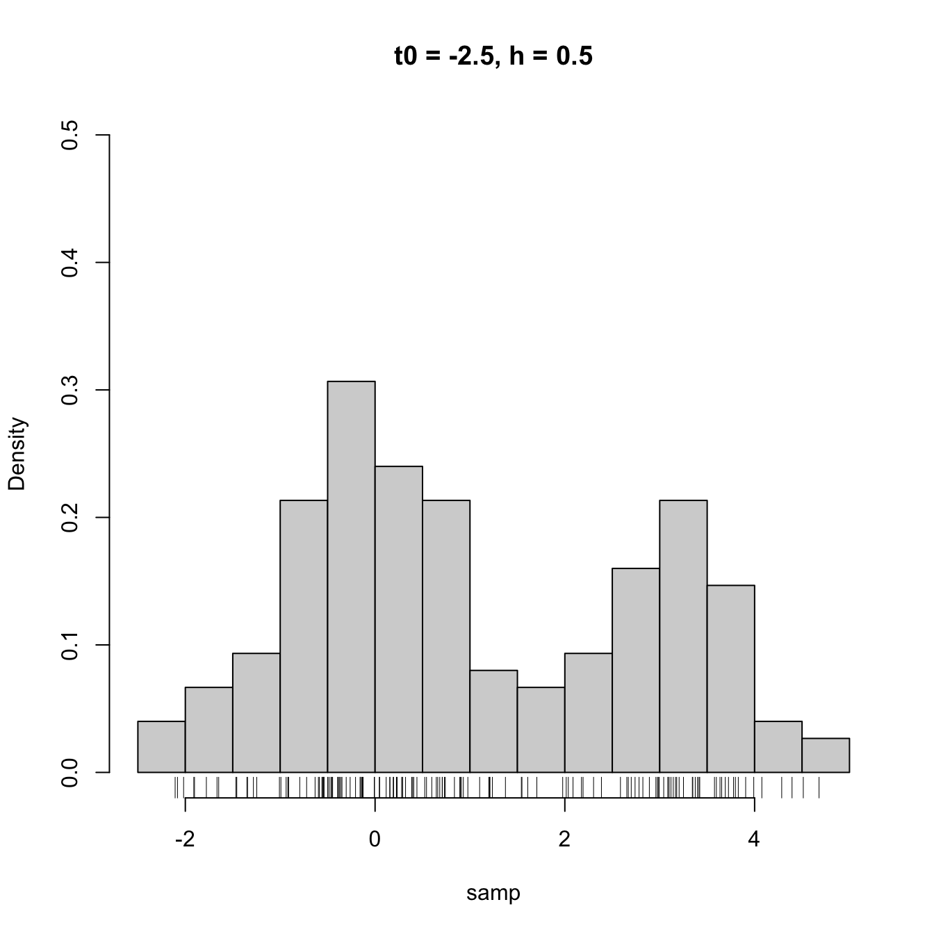

hist(samp, probability = TRUE, breaks = Bk2, ylim = c(0, 0.5),
     main = "t0 = -2.25, h = 0.5")
rug(samp)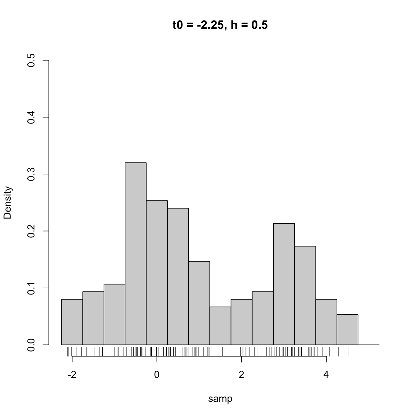

2.1.2 Moving histogram

An alternative to avoid the dependence on $t_0$ is the moving histogram or naive density estimator. The idea is to aggregate the sample $X_1,\ldots,X_n$ in intervals of the form $(x-h, x+h)$ and then use its relative frequency in $(x-h,x+h)$ to approximate the density at $x$ :

$\begin{align*} f(x)&=F'(x)\\ &=\lim_{h\to0^+}\frac{F(x+h)-F(x-h)}{2h}\\ &=\lim_{h\to0^+}\frac{\mathbb{P}[x-h<X<x+h]}{2h}. \end{align*}$

Recall the differences with the histogram: the intervals depend on the evaluation point $x$ and are centered around it. That allows to directly estimate $f(x)$ (without the proxy $f(x_0)$ ) by an estimate of the symmetric derivative.

More precisely, given a bandwidth $h>0,$ the naive density estimator builds a piecewise constant function by considering the relative frequency of $X_1,\ldots,X_n$ inside $(x-h,x+h)$ :

$\begin{align} \hat f_\mathrm{N}(x;h):=\frac{1}{2nh}\sum_{i=1}^n1_{\{x-h<X_i<x+h\}}. \tag{2.2} \end{align}$

The function has $2n$ discontinuities that are located at $X_i\pm h.$

Similarly to the histogram, the analysis of $\hat f_\mathrm{N}(x;h)$ as a random variable follows from realizing that $\sum_{i=1}^n1_{\{x-h<X_i<x+h\}}\sim \mathrm{B}(n,p_{x,h}),$ $p_{x,h}=\mathbb{P}[x-h<X<x+h]=F(x+h)-F(x-h).$ Then:

$\begin{align*} \mathbb{E}[\hat f_\mathrm{N}(x;h)]=&\,\frac{F(x+h)-F(x-h)}{2h},\\ \mathbb{V}\mathrm{ar}[\hat f_\mathrm{N}(x;h)]=&\,\frac{F(x+h)-F(x-h)}{4nh^2}\\ &-\frac{(F(x+h)-F(x-h))^2}{4nh^2}. \end{align*}$

These two results provide interesting insights on the effect of $h$ :

If $h\to0,$ then $\mathbb{E}[\hat f_\mathrm{N}(x;h)]\to f(x)$ and (2.2) is an asymptotically unbiased estimator of $f(x).$ But also $\mathbb{V}\mathrm{ar}[\hat f_\mathrm{N}(x;h)]\approx \frac{f(x)}{2nh}-\frac{f(x)^2}{n}\to\infty.$
If $h\to\infty,$ then $\mathbb{E}[\hat f_\mathrm{N}(x;h)]\to 0$ and $\mathbb{V}\mathrm{ar}[\hat f_\mathrm{N}(x;h)]\to0.$
The variance shrinks to zero if $nh\to\infty$ (or, in other words, if $h^{-1}=o(n),$ i.e. if $h^{-1}$ grows slower than $n$ ). So both the bias and the variance can be reduced if $n\to\infty,$ $h\to0,$ and $nh\to\infty,$ simultaneously.
The variance is (almost) proportional to $f(x).$

The animation in Figure 2.1 illustrates the previous points and gives insight on how the performance of (2.2) varies smoothly with $h.$

Figure 2.1: Bias and variance for the moving histogram. The animation shows how for small bandwidths the bias of $\hat f_\mathrm{N}(x;h)$ on estimating $f(x)$ is small, but the variance is high, and how for large bandwidths the bias is large and the variance is small. The variance is represented by the asymptotic $95\%$ confidence intervals for $\hat f_\mathrm{N}(x;h).$ Application also available here.

The estimator (2.2) raises an important question: Why giving the same weight to all $X_1,\ldots,X_n$ in $(x-h, x+h)$ ? After all, we are estimating $f(x)=F'(x)$ by estimating $\frac{F(x+h)-F(x-h)}{2h}$ through the relative frequency of $X_1,\ldots,X_n$ in $(x-h,x+h).$ Should not be the data points closer to $x$ more important than the ones further away? The answer to this question shows that (2.2) is indeed a particular case of a wider class of density estimators.

References

Scott, D. W. 2015. Multivariate Density Estimation. Second. Wiley Series in Probability and Statistics. Hoboken: John Wiley & Sons, Inc.

Note that it is key that the $\{B_k\}$ are deterministic (and not sample-dependent) for this result to hold.↩︎