2.5 Confidence intervals

Obtaining a Confidence Interval (CI) for $f(x)$ is a challenging task. Due to the bias results seen in Section 2.3, we know that the kde is biased for finite sample sizes, $\mathbb{E}[\hat f(x;h)]=(K_h*f)(x),$ and it is only asymptotically unbiased when $h\to0.$ This bias is called the smoothing bias and in essence complicates the obtention of CIs for $f(x),$ but not of $(K_h*f)(x).$ Let’s see with an illustrative example the differences between these two objects.

Two well-known facts for normal densities (see Appendix C in Wand and Jones (1995)) are:

$$\begin{align} (\phi_{\sigma_1}(\cdot-\mu_1)*\phi_{\sigma_2}(\cdot-\mu_2))(x)&=\phi_{(\sigma_1^2+\sigma_2^2)^{1/2}}(x-\mu_1-\mu_2),\tag{2.23}\\ \int\phi_{\sigma_1}(x-\mu_1)\phi_{\sigma_2}(x-\mu_2)\,\mathrm{d}x&=\phi_{(\sigma_1^2+\sigma_2^2)^{1/2}}(\mu_1-\mu_2),\\ \phi_{\sigma}(x-\mu)^r&=\frac{1}{\sigma^{r-1}}(2\pi)^{(1-r)/2}\phi_{\sigma/ r^{1/2}}(x-\mu)\frac{1}{r^{1/2}}.\tag{2.24} \end{align}$$

As a consequence, if $K=\phi$ (i.e., $K_h=\phi_h$) and $f(\cdot)=\phi_\sigma(\cdot-\mu),$ we have that

$$\begin{align} (K_h*f)(x)&=\phi_{(h^2+\sigma^2)^{1/2}}(x-\mu),\tag{2.25}\\ (K_h^2*f)(x)&=\left(\frac{1}{(2\pi)^{1/2}h}\phi_{h/2^{1/2}}/2^{1/2}*f\right)(x)\nonumber\\ &=\frac{1}{2\pi^{1/2}h}\left(\phi_{h/2^{1/2}}*f\right)(x)\nonumber\\ &=\frac{1}{2\pi^{1/2}h}\phi_{(h^2/2+\sigma^2)^{1/2}}(x-\mu).\tag{2.26} \end{align}$$

Thus, the exact expectation of the kde for estimating the density of a $\mathcal{N}(\mu,\sigma^2)$ is the density of a $\mathcal{N}(\mu,\sigma^2+h^2).$ Clearly, when $h\to0,$ the bias disappears. Removing this finite-sample size bias is not simple: if the bias is expanded, $f''$ appears. Thus for attempting to unbias $\hat f(\cdot;h)$ we have to estimate $f'',$ which is a harder task than estimating $f$! Taking second derivatives on the kde does not simply work out-of-the-box, since the bandwidths for estimating $f$ and $f''$ scale differently. We refer the interested reader to Section 2.12 in Wand and Jones (1995) for a quick review of derivative kde.

The previous deadlock can be solved if we limit our ambitions. Rather than constructing a confidence interval for $f(x),$ we will do it for $\mathbb{E}[\hat f(x;h)]=(K_h*f)(x).$ There is nothing wrong with this, as long as we are careful when we report the results to make it clear that the CI is for $(K_h*f)(x)$ and not $f(x).$

The building block for the CI for $\mathbb{E}[\hat f(x;h)]=(K_h*f)(x)$ is Theorem 2.2, which stated that:

$$\begin{align*} \sqrt{nh}(\hat f(x;h)-\mathbb{E}[\hat f(x;h)])\stackrel{d}{\longrightarrow}\mathcal{N}(0,R(K)f(x)). \end{align*}$$

Plugging-in $\hat f(x;h)=f(x)+O_\mathbb{P}(h^2+(nh)^{-1})=f(x)(1+o_\mathbb{P}(1))$ (see Exercise 2.8) as an estimate for $f(x)$ in the variance, we have by the Slutsky’s theorem that

$$\begin{align*} \sqrt{\frac{nh}{R(K)\hat f(x;h)}}&(\hat f(x;h)-\mathbb{E}[\hat f(x;h)])\\ &=\sqrt{\frac{nh}{R(K)f(x)}}(\hat f(x;h)-\mathbb{E}[\hat f(x;h)])(1+o_\mathbb{P}(1))\\ &\stackrel{d}{\longrightarrow}\mathcal{N}(0,1). \end{align*}$$

Therefore, an asymptotic $100(1-\alpha)\%$ confidence interval for $\mathbb{E}[\hat f(x;h)]$ that can be straightforwardly computed is:

$$\begin{align} I=\left(\hat f(x;h)\pm z_{\alpha}\sqrt{\frac{R(K)\hat f(x;h)}{nh}}\right).\tag{2.27} \end{align}$$

Recall that if we wanted to do obtain a CI with the second result in Theorem 2.2 we will need to estimate $f''(x).$

Remark. Several points regarding the CI require proper awareness:

1. The CI is for $\mathbb{E}[\hat f(x;h)]=(K_h*f)(x),$ not $f(x).$
2. The CI is pointwise. That means that $\mathbb{P}\left[\mathbb{E}[\hat f(x;h)]\in I\right]\approx 1-\alpha$ for each $x\in\mathbb{R},$ but not simultaneously. This is,$\mathbb{P}\left[\mathbb{E}[\hat f(x;h)]\in I,\,\forall x\in\mathbb{R}\right]\neq 1-\alpha.$
3. We are approximating $f(x)$ in the variance by $\hat f(x;h)=f(x)+O_\mathbb{P}(h^2+(nh)^{-1}).$ Additionally, the convergence to a normal distribution happens at rate $\sqrt{nh}.$ Hence both $h$ and $nh$ need to small and large, respectively, for a good coverage.
4. The CI is for a deterministic bandwidth $h$ (i.e., not selected from the sample), which is not usually the case in practice. If a bandwidth selector is employed, the coverage may be affected, specially for small $n.$

We illustrate the construction of the CI in (2.27) for the situation where the reference density is a $\mathcal{N}(\mu,\sigma^2)$ and the normal kernel is employed. This allows to use (2.25) and (2.26) in combination with (2.6) and (2.7) to obtain:

$$\begin{align*} \mathbb{E}[\hat f(x;h)]&=\phi_{(h^2+\sigma^2)^{1/2}}(x-\mu),\\ \mathbb{V}\mathrm{ar}[\hat f(x;h)]&=\frac{1}{n}\left(\frac{\phi_{(h^2/2+\sigma^2)^{1/2}}(x-\mu)}{2\pi^{1/2}h}-(\phi_{(h^2+\sigma^2)^{1/2}}(x-\mu))^2\right). \end{align*}$$

The following piece of code evaluates the proportion of times that $\mathbb{E}[\hat f(x;h)]$ belongs to $I$ for each $x\in\mathbb{R},$ both estimating and knowing the variance in the asymptotic distribution.

# R(K) for a normal
Rk <- 1 / (2 * sqrt(pi))

# Generate a sample from a N(mu, sigma^2)
n <- 100
mu <- 0
sigma <- 1
set.seed(123456)
x <- rnorm(n = n, mean = mu, sd = sigma)

# Compute the kde (NR bandwidth)
kde <- density(x = x, from = -4, to = 4, n = 1024, bw = "nrd")

# Selected bandwidth
h <- kde$bw

# Estimate the variance
hatVarKde <- kde$y * Rk / (n * h)

# True expectation and variance (because the density is a normal)
EKh <- dnorm(x = kde$x, mean = mu, sd = sqrt(sigma^2 + h^2))
varKde <- (dnorm(kde$x, mean = mu, sd = sqrt(h^2 / 2 + sigma^2)) /
             (2 * sqrt(pi) * h) - EKh^2) / n

# CI with estimated variance
alpha <- 0.05
zalpha <- qnorm(1 - alpha/2)
ciLow1 <- kde$y - zalpha * sqrt(hatVarKde)
ciUp1 <- kde$y + zalpha * sqrt(hatVarKde)

# CI with known variance
ciLow2 <- kde$y - zalpha * sqrt(varKde)
ciUp2 <- kde$y + zalpha * sqrt(varKde)

# Plot estimate, CIs and expectation
plot(kde, main = "Density and CIs", ylim = c(0, 1))
lines(kde$x, ciLow1, col = "gray")
lines(kde$x, ciUp1, col = "gray")
lines(kde$x, ciUp2, col = "gray", lty = 2)
lines(kde$x, ciLow2, col = "gray", lty = 2)
lines(kde$x, EKh, col = "red")
legend("topright", legend = c("Estimate", "CI estimated var",
                              "CI known var", "Smoothed density"),
       col = c("black", "gray", "gray", "red"), lwd = 2, lty = c(1, 1, 2, 1))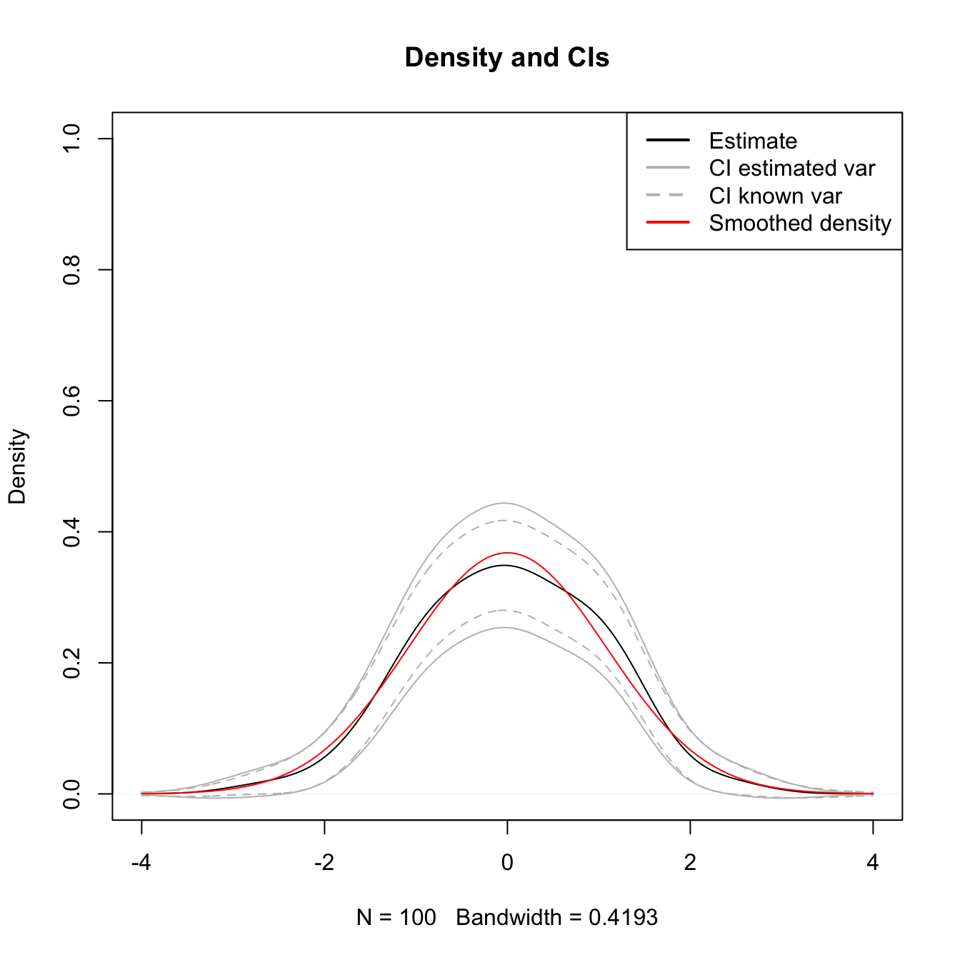

The above code computes the CI. But it does not show any insight on the effective coverage of the CI. The next simulation exercise tackles with this issue.

# Simulation setting
n <- 100; h <- 0.2
mu <- 0; sigma <- 1 # Normal parameters
M <- 5e2 # Number of replications in the simulation
nGrid <- 512 # Number of x's for computing the kde
alpha <- 0.05; zalpha <- qnorm(1 - alpha/2) # alpha for CI

# Compute expectation and variance
kde <- density(x = 0, bw = h, from = -4, to = 4, n = nGrid) # Just to get kde$x
EKh <- dnorm(x = kde$x, mean = mu, sd = sqrt(sigma^2 + h^2))
varKde <- (dnorm(kde$x, mean = mu, sd = sqrt(h^2 / 2 + sigma^2)) /
           (2 * sqrt(pi) * h) - EKh^2) / n

# For storing if the mean is inside the CI
insideCi1 <- insideCi2 <- matrix(nrow = M, ncol = nGrid)

# Simulation
set.seed(12345)
for (i in 1:M) {

  # Sample & kde
  x <- rnorm(n = n, mean = mu, sd = sigma)
  kde <- density(x = x, bw = h, from = -4, to = 4, n = nGrid)
  hatSdKde <- sqrt(kde$y * Rk / (n * h))

  # CI with estimated variance
  ciLow1 <- kde$y - zalpha * hatSdKde
  ciUp1 <- kde$y + zalpha * hatSdKde

  # CI with known variance
  ciLow2 <- kde$y - zalpha * sqrt(varKde)
  ciUp2 <- kde$y + zalpha * sqrt(varKde)

  # Check if for each x the mean is inside the CI
  insideCi1[i, ] <- EKh > ciLow1 & EKh < ciUp1
  insideCi2[i, ] <- EKh > ciLow2 & EKh < ciUp2

}

# Plot results
plot(kde$x, colMeans(insideCi1), ylim = c(0.25, 1), type = "l",
     main = "Coverage CIs", xlab = "x", ylab = "Coverage")
lines(kde$x, colMeans(insideCi2), col = 4)
abline(h = 1 - alpha, col = 2)
abline(h = 1 - alpha + c(-1, 1) * qnorm(0.975) *
         sqrt(alpha * (1 - alpha) / M), col = 2, lty = 2)
legend(x = "bottom", legend = c("CI estimated var", "CI known var",
                                "Nominal level",
                                "95% CI for the nominal level"),
       col = c(1, 4, 2, 2), lwd = 2, lty = c(1, 1, 1, 2))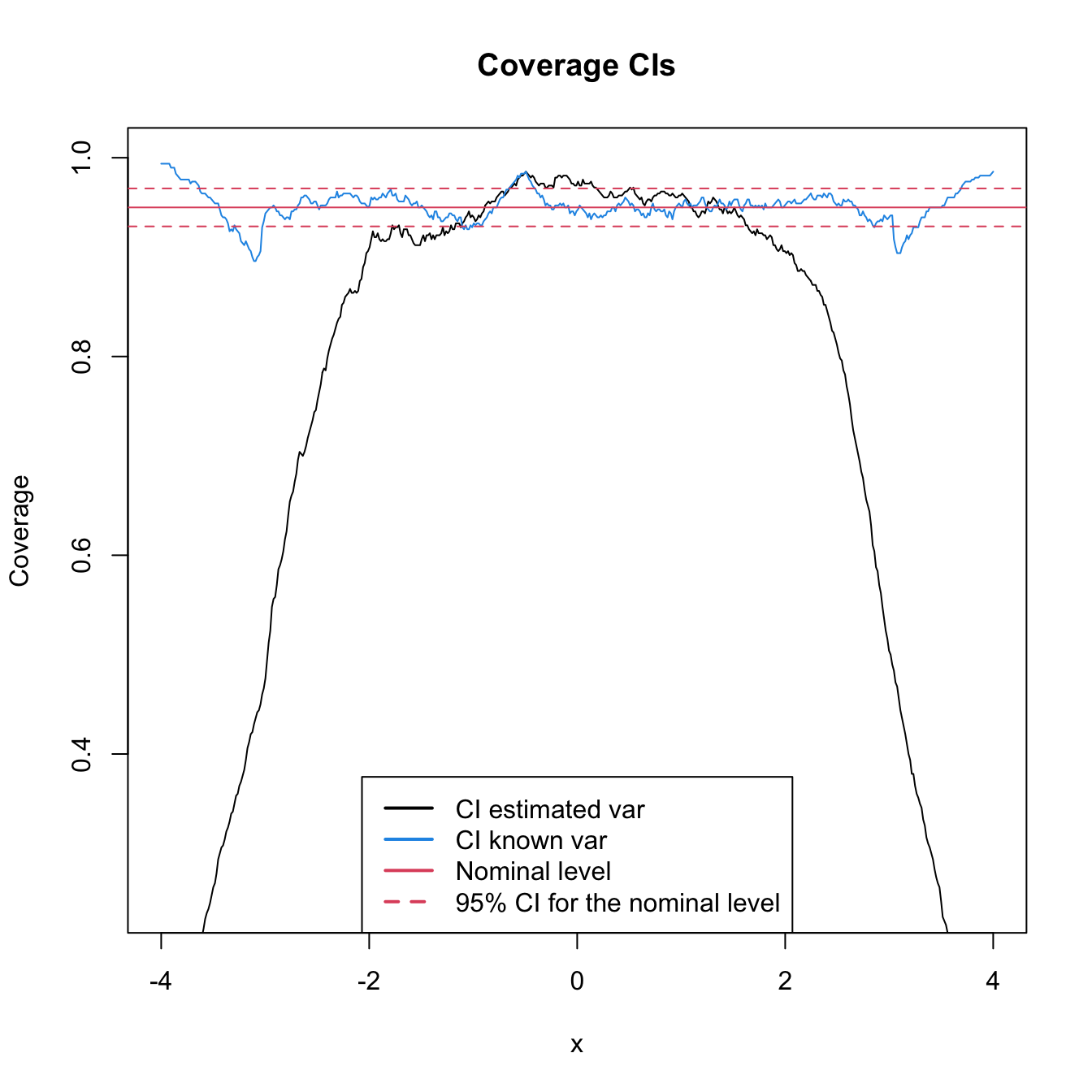

Exercise 2.3 Explore the coverage of the asymptotic CI for varying values of $h.$ To that end, adapt the previous code to work in a manipulate environment like the example given below.

# Load manipulate
# install.packages("manipulate")
library(manipulate)

# Sample
x <- rnorm(100)

# Simple plot of kde for varying h
manipulate({

  kde <- density(x = x, from = -4, to = 4, bw = h)
  plot(kde, ylim = c(0, 1), type = "l", main = "")
  curve(dnorm(x), from = -4, to = 4, col = 2, add = TRUE)
  rug(x)

}, h = slider(min = 0.01, max = 2, initial = 0.5, step = 0.01))

References

Wand, M. P., and M. C. Jones. 1995. Kernel Smoothing. Vol. 60. Monographs on Statistics and Applied Probability. London: Chapman & Hall, Ltd. https://doi.org/10.1007/978-1-4899-4493-1.