3.5 Local likelihood
We explore in this section an extension of the local polynomial estimator. This extension aims to estimate the regression function by relying in the likelihood, rather than the least squares. Thus, the idea behind the local likelihood is to fit, locally, parametric models by maximum likelihood.
We begin by seeing that local likelihood using the the linear model is equivalent to local polynomial modelling. Theorem 3.1 showed that, under the assumptions given in Section 3.1.1, the maximum likelihood estimate of \(\boldsymbol{\beta}\) in the linear model
\[\begin{align} Y|(X_1,\ldots,X_p)\sim\mathcal{N}(\beta_0+\beta_1X_1+\cdots+\beta_pX_p,\sigma^2)\tag{3.25} \end{align}\]
was equivalent to the least squares estimate, \(\hat{\boldsymbol{\beta}}_\mathrm{ML}=(\mathbf{X}'\mathbf{X})^{-1}\mathbf{X}\mathbf{Y}.\) The reason was the form of the conditional (on \(X_1,\ldots,X_p\)) likelihood:
\[\begin{align*} \ell(\boldsymbol{\beta})=&\,-\frac{n}{2}\log(2\pi\sigma^2)\nonumber\\ &-\frac{1}{2\sigma^2}\sum_{i=1}^n(Y_i-\beta_0-\beta_1X_{i1}-\cdots-\beta_pX_{ip})^2. \end{align*}\]
If there is a single predictor \(X,\) polynomial fitting of order \(p\) of the conditional meal can be achieved by the well-known trick of identifying the \(j\)-th predictor \(X_j\) in (3.25) by \(X^j.\) This results in
\[\begin{align} Y|X\sim\mathcal{N}(\beta_0+\beta_1X+\cdots+\beta_pX^p,\sigma^2).\tag{3.26} \end{align}\]
Therefore, maximizing with respect to \(\boldsymbol{\beta}\) the weighted log-likelihood of the linear model around \(x\) of (3.26),
\[\begin{align*} \ell_{x,h}(\boldsymbol{\beta})=&\,-\frac{n}{2}\log(2\pi\sigma^2)\\ &-\frac{1}{2\sigma^2}\sum_{i=1}^n(Y_i-\beta_0-\beta_1X_i-\cdots-\beta_pX_i^p)^2K_h(x-X_i), \end{align*}\]
provides \(\hat\beta_0=\hat m(x;p,h),\) the local polynomial estimator, as it was obtained in (3.17).
The same idea can be applied for other parametric models. The family of generalized linear models15, which presents an extension of the linear model to different kinds of response variables, provides a particularly convenient parametric framework. Generalized linear models are constructed by mapping the support of \(Y\) to \(\mathbb{R}\) by a link function \(g,\) and then modeling the transformed expectation by a linear model. Thus, a generalized linear model for the predictors \(X_1,\ldots,X_p,\) assumes
\[\begin{align*} g\left(\mathbb{E}[Y|X_1=x_1,\ldots,X_p=x_p]\right)&=\beta_0+\beta_1x_1+\cdots+\beta_px_p \end{align*}\]
or, equivalently,
\[\begin{align*} \mathbb{E}[Y|X_1=x_1,\ldots,X_p=x_p]&=g^{-1}\left(\beta_0+\beta_1x_1+\cdots+\beta_px_p\right) \end{align*}\]
together with a distribution assumption for \(Y|(X_1,\ldots,X_p).\) The following table lists some useful transformations and distributions that are adequate to model responses in different supports. Recall that the linear and logistic models of Sections 3.1.1 and 3.1.2 are obtained from the first and second rows, respectively.
| Support of \(Y\) | Distribution | Link \(g(\mu)\) | \(g^{-1}(\eta)\) | \(Y\vert(X_1=x_1,\ldots,X_p=x_p)\) |
|---|---|---|---|---|
| \(\mathbb{R}\) | \(\mathcal{N}(\mu,\sigma^2)\) | \(\mu\) | \(\eta\) | \(\mathcal{N}(\beta_0+\beta_1x_1+\cdots+\beta_px_p,\sigma^2)\) |
| \((0,\infty)\) | \(\mathrm{Exp}(\lambda)\) | \(\mu^{-1}\) | \(\eta^{-1}\) | \(\mathrm{Exp}(\beta_0+\beta_1x_1+\cdots+\beta_px_p)\) |
| \(0,1\) | \(\mathrm{B}(1,p)\) | \(\mathrm{logit}(\mu)\) | \(\mathrm{logistic}(\eta)\) | \(\mathrm{B}\left(1,\mathrm{logistic}(\beta_0+\beta_1x_1+\cdots+\beta_px_p)\right)\) |
| \(0,1,2,\ldots\) | \(\mathrm{Pois}(\lambda)\) | \(\log(\mu)\) | \(e^\eta\) | \(\mathrm{Pois}(e^{\beta_0+\beta_1x_1+\cdots+\beta_px_p})\) |
All the distributions of the table above are members of the exponential family of distributions, which is the family of distributions with pdf expressible as
\[\begin{align*} f(y;\theta,\phi)=\exp\left\{\frac{y\theta-b(\theta)}{a(\phi)}+c(y,\phi)\right\}, \end{align*}\]
where \(a(\cdot),\) \(b(\cdot),\) and \(c(\cdot,\cdot)\) are specific functions, \(\phi\) is the scale parameter and \(\theta\) is the canonical parameter. If the canonical link function \(g\) (the ones in the table above are all) is employed, then \(\theta=g(\mu)\) and s a consequence
\[\begin{align*} \theta(x_1,\ldots,x_p):=g(\mathbb{E}[Y|X_1=x_1,\ldots,X_p=x_p]). \end{align*}\]
Recall that, again, if there is only one predictor, identifying the \(j\)-th predictor \(X_j\) by \(X^j\) in the above expressions allows to consider \(p\)-th order polynomial fits for \(g\left(\mathbb{E}[Y|X_1=x_1,\ldots,X_p=x_p]\right).\)
Figure 3.7: Construction of the local likelihood estimator. The animation shows how local likelihood fits in a neighborhood of \(x\) are combined to provide an estimate of the regression function for binary response, which depends on the polynomial degree, bandwidth, and kernel (gray density at the bottom). The data points are shaded according to their weights for the local fit at \(x.\) Application also available here.
We illustrate the local likelihood principle for the logistic regression, the simplest non-linear model. In this case, \((X_1,Y_1),\ldots,(X_n,Y_n)\) with
\[\begin{align*} Y_i|X_i\sim \mathrm{Ber}(p(X_i)),\quad i=1,\ldots,n. \end{align*}\]
for \(p(x)=\mathbb{P}[Y=1|X=x]=\mathbb{E}[Y|X=x].\) The link function is \(g(x)=\mathrm{logit}(x)=\log\left(\frac{x}{1-x}\right)\) and \(\theta(x)=\mathrm{logit}(p(x)).\) Assuming that \(\theta(x)=\beta_0+\beta_1x+\cdots+\beta_px^p\,\)16, we have that the log-likelihood of \(\boldsymbol{\beta}\) is
\[\begin{align*} \ell(\boldsymbol{\beta}) =&\,\sum_{i=1}^n\left\{Y_i\log(\mathrm{logistic}(\theta(X_i)))+(1-Y_i)\log(1-\mathrm{logistic}(\theta(X_i)))\right\}\nonumber\\ =&\,\sum_{i=1}^n\ell(Y_i,\theta(X_i)), \end{align*}\]
where we consider the log-likelihood addend
\[\begin{align*} \ell(y,\theta)=y\theta-\log(1+e^\theta) \end{align*}\]
and make explicit the dependence on \(\theta(x)\) for clarity in the next developments, and implicit the dependence on \(\boldsymbol{\beta}.\) The local log-likelihood of \(\boldsymbol{\beta}\) around \(x\) is then
\[\begin{align} \ell_{x,h}(\boldsymbol{\beta}) =\sum_{i=1}^n\ell(Y_i,\theta(X_i-x))K_h(x-X_i).\tag{3.27} \end{align}\]
Maximizing17 the local log-likelihood (3.27) with respect to \(\boldsymbol{\beta}\) provides
\[\begin{align*} \hat{\boldsymbol{\beta}}=\arg\max_{\boldsymbol{\beta}\in\mathbb{R}^{p+1}}\ell_{x,h}(\boldsymbol{\beta}). \end{align*}\]
The local likelihood estimate of \(\theta(x)\) is
\[\begin{align*} \hat\theta(x):=\hat\beta_0. \end{align*}\]
Note that the dependence of \(\hat\beta_0\) on \(x\) and \(h\) is omitted. From \(\hat\theta(x),\) we can obtain the local logistic regression evaluated at \(x\) as
\[\begin{align} \hat m_{\ell}(x;h,p):=g^{-1}\left(\hat\theta(x)\right)=\mathrm{logistic}(\hat\beta_0).\tag{3.28} \end{align}\]
The code below shows three different ways of implementing the local logistic regression (of first degree) in R.
# Simulate some data
n <- 200
logistic <- function(x) 1 / (1 + exp(-x))
p <- function(x) logistic(1 - 3 * sin(x))
set.seed(123456)
X <- runif(n = n, -3, 3)
Y <- rbinom(n = n, size = 1, prob = p(X))

# Set bandwidth and evaluation grid
h <- 0.25
x <- seq(-3, 3, l = 501)

# Optimize the weighted log-likelihood through glm's built in procedure
suppressWarnings(
  fitGlm <- sapply(x, function(x) {
    K <- dnorm(x = x, mean = X, sd = h)
    glm.fit(x = cbind(1, X - x), y = Y, weights = K,
            family = binomial())$coefficients[1]
  })
)

# Optimize the weighted log-likelihood explicitly
suppressWarnings(
  fitNlm <- sapply(x, function(x) {
    K <- dnorm(x = x, mean = X, sd = h)
    nlm(f = function(beta) {
      -sum(K * (Y * (beta[1] + beta[2] * (X - x)) -
                  log(1 + exp(beta[1] + beta[2] * (X - x)))))
      }, p = c(0, 0))$estimate[1]
  })
)

# Using locfit
# Bandwidth can not be controlled explicitly - only though nn in ?lp
library(locfit)
fitLocfit <- locfit(Y ~ lp(X, deg = 1, nn = 0.25), family = "binomial",
                    kern = "gauss")

# Compare fits
plot(x, p(x), ylim = c(0, 1.5), type = "l", lwd = 2)
lines(x, logistic(fitGlm), col = 2)
lines(x,logistic(fitNlm), col = 3, lty = 2)
plot(fitLocfit, add = TRUE, col = 4)
legend("topright", legend = c("p(x)", "glm", "nlm", "locfit"), lwd = 2,
       col = c(1, 2, 3, 4), lty = c(1, 1, 2, 1))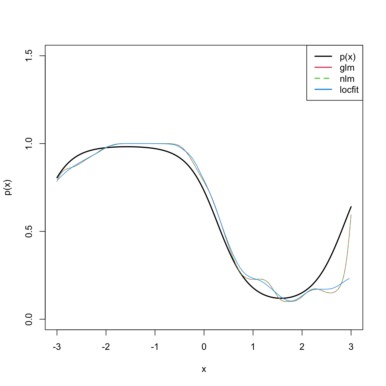
Bandwidth selection can be done by means of likelihood cross-validation. The objective is to maximize the local likelihood fit at \((X_i,Y_i)\) but removing the influence by the datum itself. That is, maximizing
\[\begin{align} \mathrm{LCV}(h)=\sum_{i=1}^n\ell(Y_i,\hat\theta_{-i}(X_i)),\tag{3.29} \end{align}\]
where \(\hat\theta_{-i}(X_i)\) represents the local fit at \(X_i\) without the \(i\)-th datum \((X_i,Y_i).\) Unfortunately, the nonlinearity of (3.28) forbids a simplifying result as Proposition 3.1. Thus, in principle, it is required to fit \(n\) local likelihoods for sample size \(n-1\) for obtaining a single evaluation of (3.29).
There is, however, an approximation (see Sections 4.3.3 and 4.4.3 of Loader (1999)) to (3.29) that only requires a local likelihood fit for a single sample. We sketch its basis as follows, without aiming to go in full detail. The approximation considers the first and second derivatives of \(\ell(y,\theta)\) with respect to \(\theta,\) \(\dot{\ell}(y,\theta)\) and \(\ddot{\ell}(y,\theta).\) In the case of the logistic model, these are:
\[\begin{align*} \dot{\ell}(y,\theta)&=y-\mathrm{logistic}(\theta),\\ \ddot{\ell}(y,\theta)&=-\mathrm{logistic}(\theta)(1 - \mathrm{logistic}(\theta)). \end{align*}\]
It can be seen that (Exercise 4.6 in Loader (1999))
\[\begin{align} \hat\theta_{-i}(X_i)\approx\hat\theta(X_i)-\mathrm{infl}(X_i)\left(\dot{l}(Y_i,\hat\theta(X_i))\right)^2,\tag{3.30} \end{align}\]
where \(\hat\theta(X_i)\) represents the local fit at \(X_i\) and the influence function is defined as (page 75 of Loader (1999))
\[\begin{align*} \mathrm{infl}(x):=\mathbf{e}_1'(\mathbf{X}_x'\mathbf{W}_x\mathbf{V}\mathbf{X}_x)^{-1}\mathbf{e}_1K(0) \end{align*}\]
for the matrices
\[\begin{align*} \mathbf{X}_x:=\begin{pmatrix} 1 & X_1-x & \cdots & (X_1-x)^p/p!\\ \vdots & \vdots & \ddots & \vdots\\ 1 & X_n-x & \cdots & (X_n-x)^p/p!\\ \end{pmatrix}_{n\times(p+1)} \end{align*}\]
and
\[\begin{align*} \mathbf{W}_x&:=\mathrm{diag}(K_h(X_1-x),\ldots, K_h(X_n-x)),\\ \mathbf{V}&:=-\mathrm{diag}(\ddot{l}(Y_1,\theta(X_1)),\ldots, \ddot{l}(Y_n,\theta(X_n))). \end{align*}\]
A one-term Taylor expansion of \(\ell(Y_i,\hat\theta_{-i}(X_i))\) using (3.30) gives
\[\begin{align*} \ell(Y_i,\hat\theta_{-i}(X_i))=\ell(Y_i,\hat\theta(X_i))-\mathrm{infl}(X_i)\left(\dot{\ell}(Y_i,\theta(X_i))\right)^2. \end{align*}\]
Therefore:
\[\begin{align*} \mathrm{LCV}(h)&=\sum_{i=1}^n\ell(Y_i,\hat\theta_{-i}(X_i))\\ &\approx\sum_{i=1}^n\ell(Y_i,\hat\theta(X_i))+\mathrm{infl}(X_i)\left(\dot{\ell}(Y_i,\hat\theta(X_i))\right)^2. \end{align*}\]
Recall that \(\theta(X_i)\) are unknown and hence they must be estimated.
We conclude by illustrating how to compute the LCV function and optimize it (keep in mind that much more efficient implementations are possible!).
# Exact LCV - recall that we *maximize* the LCV!
h <- seq(0.1, 2, by = 0.1)
suppressWarnings(
  LCV <- sapply(h, function(h) {
  sum(sapply(1:n, function(i) {
    K <- dnorm(x = X[i], mean = X[-i], sd = h)
    nlm(f = function(beta) {
      -sum(K * (Y[-i] * (beta[1] + beta[2] * (X[-i] - X[i])) -
                  log(1 + exp(beta[1] + beta[2] * (X[-i] - X[i])))))
      }, p = c(0, 0))$minimum
    }))
  })
)
plot(h, LCV, type = "o")
abline(v = h[which.max(LCV)], col = 2)