2.3 Asymptotic properties
Asymptotic results give us insights on the large-sample (\(n\to\infty\)) properties of an estimator. One might think why are they useful, since in practice we only have finite sample sizes. Apart from purely theoretical reasons, asymptotic results usually give highly valuable insights on the properties of the method, typically simpler than finite-sample results (which might be analytically untractable).
Along this section we will make the following assumptions:
- A1. The density \(f\) is twice continuously differentiable and the second derivative is square integrable.
- A2. The kernel \(K\) is a symmetric and bounded pdf with finite second moment and square integrable.
- A3. \(h=h_n\) is a deterministic sequence of bandwidths6 such that, when \(n\to\infty,\) \(h\to0\) and \(nh\to\infty.\)
We need to introduce some notation. From now on, the integrals are thought to be over \(\mathbb{R},\) if not stated otherwise. The second moment of the kernel is denoted as \(\mu_2(K):=\int z^2K(z)\,\mathrm{d}z.\) The squared integral of a function \(f,\) is denoted by \(R(f):=\int f(x)^2\,\mathrm{d}x.\) The convolution between two real functions \(f\) and \(g,\) \(f*g,\) is the function
\[\begin{align} (f*g)(x):=\int f(x-y)g(y)\,\mathrm{d}y=(g*f)(x).\tag{2.5} \end{align}\]
We are now ready to obtain the bias and variance of \(\hat f(x;h).\) Recall that is not possible to apply the “binomial trick” we used previously since now the estimator is not piecewise constant. Instead of that, we use the linearity of the kde and the convolution definition. For the bias, recall that
\[\begin{align} \mathbb{E}[\hat f(x;h)]&=\frac{1}{n}\sum_{i=1}^n\mathbb{E}[K_h(x-X_i)]\nonumber\\ &=\int K_h(x-y)f(y)\,\mathrm{d}y\nonumber\\ &=(K_h * f)(x).\tag{2.6} \end{align}\]
Similarly, the variance is obtained as
\[\begin{align} \mathbb{V}\mathrm{ar}[\hat f(x;h)]&=\frac{1}{n}((K_h^2*f)(x)-(K_h*f)^2(x)).\tag{2.7} \end{align}\]
These two expressions are exact, but they are hard to interpret. Equation (2.6) indicates that the estimator is biased (we will see an example of that bias in Section 2.5), but it does not differentiate explicitly the effects of kernel, bandwidth and density on the bias. The same happens with (2.7), yet more emphasized. That is why the following asymptotic expressions are preferred.
Theorem 2.1 Under A1–A3, the bias and variance of the kde at \(x\) are
\[\begin{align} \mathrm{Bias}[\hat f(x;h)]&=\frac{1}{2}\mu_2(K)f''(x)h^2+o(h^2),\tag{2.8}\\ \mathbb{V}\mathrm{ar}[\hat f(x;h)]&=\frac{R(K)}{nh}f(x)+o((nh)^{-1}).\tag{2.9} \end{align}\]
Proof. For the bias we consider the change of variables \(z=\frac{x-y}{h},\) \(y=x-hz,\) \(\,\mathrm{d}y=-h\,\mathrm{d}z.\) The integral limits flip and we have:
\[\begin{align} \mathbb{E}[\hat f(x;h)]&=\int K_h(x-y)f(y)\,\mathrm{d}y\nonumber\\ &=\int K(z)f(x-hz)\,\mathrm{d}z.\tag{2.10} \end{align}\]
Since \(h\to0,\) an application of a second-order Taylor expansion gives
\[\begin{align} f(x-hz)=&\,f(x)+f'(x)hz+\frac{f''(x)}{2}h^2z^2\\ &+o(h^2z^2). \tag{2.11} \end{align}\]
Substituting (2.11) in (2.10), and bearing in mind that \(K\) is a symmetric density around \(0,\) we have
\[\begin{align*} \int K(z)&f(x-hz)\,\mathrm{d}z\\ =&\,\int K(z)\Big\{f(x)+f'(x)hz+\frac{f''(x)}{2}h^2z^2\\ &+o(h^2z^2)\Big\}\,\mathrm{d}z\\ =&\,f(x)+\frac{1}{2}\mu_2(K)f''(x)h^2+o(h^2), \end{align*}\]
which provides (2.8).
For the variance, first note that
\[\begin{align} \mathbb{V}\mathrm{ar}[\hat f(x;h)]&=\frac{1}{n^2}\sum_{i=1}^n\mathbb{V}\mathrm{ar}[K_h(x-X_i)]\nonumber\\ &=\frac{1}{n}\left\{\mathbb{E}[K_h^2(x-X)]-\mathbb{E}[K_h(x-X)]^2\right\}. \tag{2.12} \end{align}\]
The second term of (2.12) is already computed, so we focus on the first. Using the previous change of variables and a first-order Taylor expansion, we have:
\[\begin{align} \mathbb{E}[K_h^2(x-X)]&=\frac{1}{h}\int K^2(z)f(x-hz)\,\mathrm{d}z\nonumber\\ &=\frac{1}{h}\int K^2(z)\left\{f(x)+O(hz)\right\}\,\mathrm{d}z\nonumber\\ &=\frac{R(K)}{h}f(x)+O(1). \tag{2.13} \end{align}\]
Plugging-in (2.12) into (2.13) gives
\[\begin{align*} \mathbb{V}\mathrm{ar}[\hat f(x;h)]&=\frac{1}{n}\left\{\frac{R(K)}{h}f(x)+O(1)-O(1)\right\}\\ &=\frac{R(K)}{nh}f(x)+O(n^{-1})\\ &=\frac{R(K)}{nh}f(x)+o((nh)^{-1}), \end{align*}\]
since \(n^{-1}=o((nh)^{-1}).\)
Remark. Integrating little-\(o\)’s is a tricky issue. In general, integrating a \(o^x(1)\) quantity, possibly dependent on \(x,\) does not provide an \(o(1).\) In other words: \(\int o^x(1)\,\mathrm{d}x\neq o(1).\) If the previous hold with equality, then the limits and integral will be interchangeable. But this is not always true – only if certain conditions are met; recall the dominated convergence theorem (Theorem 1.12). If one wants to be completely rigorous on the two implicit commutations of integrals and limits that took place in the proof, it is necessary to have explicit control of the remainder via Taylor’s theorem (Theorem 1.11) and then apply the dominated convergence theorem. For simplicity in the exposition, we avoid this.
The bias and variance expressions (2.8) and (2.9) yield interesting insights (see Figure 2.1 for their visualization):
The bias decreases with \(h\) quadratically. In addition, the bias at \(x\) is directly proportional to \(f''(x).\) This has an interesting interpretation:
- The bias is negative in concave regions, i.e. \(\{x\in\mathbb{R}:f''(x)<0\}.\) These regions correspod to peaks and modes of \(f\), where the kde underestimates \(f\) (tends to be below \(f\)).
- Conversely, the bias is positive in convex regions, i.e. \(\{x\in\mathbb{R}:f''(x)>0\}.\) These regions correspod to valleys and tails of \(f\), where the kde overestimates \(f\) (tends to be above \(f\)).
- The wilder the curvature \(f'',\) the harder to estimate \(f\). Flat density regions are easier to estimate than wiggling regions with high curvature (several modes).
The variance depends directly on \(f(x).\) The higher the density, the more variable is the kde. Interestingly, the variance decreases as a factor of \((nh)^{-1},\) a consequence of \(nh\) playing the role of the effective sample size for estimating \(f(x).\) The density at \(x\) is not estimated using all the sample points, but only a fraction proportional to \(nh\) in a neighborhood of \(x.\)
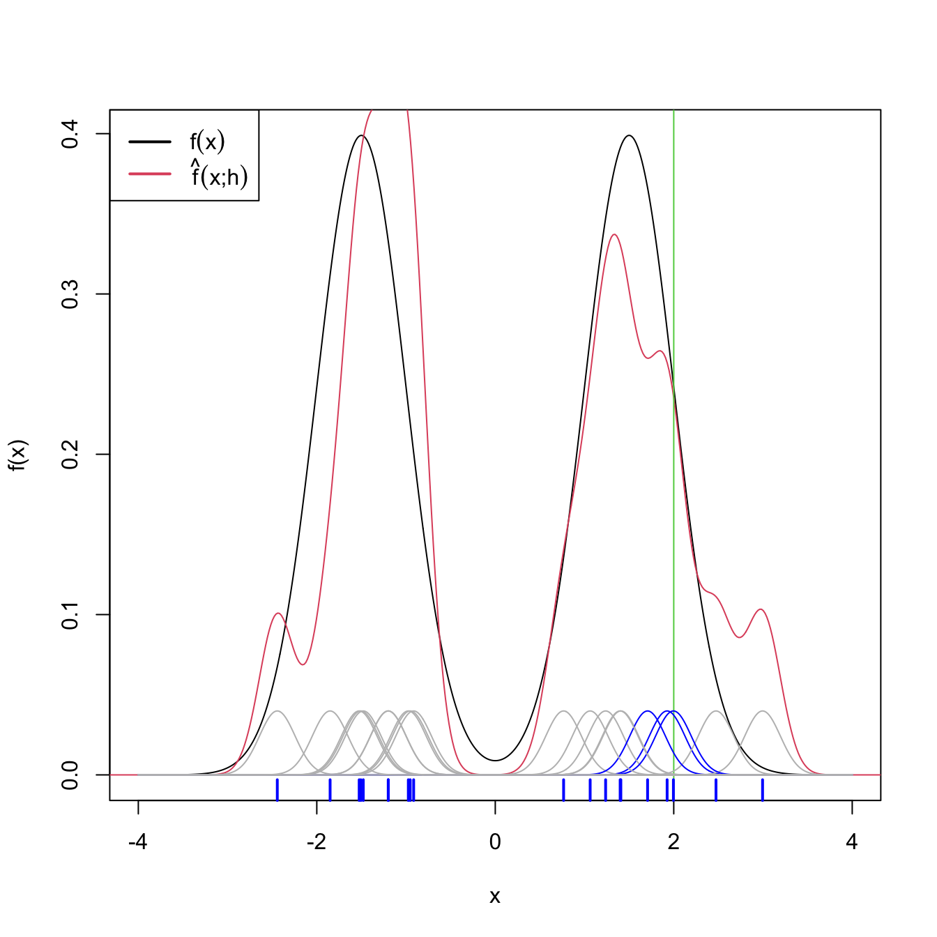
Figure 2.3: Illustration of the effective sample size for estimating \(f(x)\) at \(x=2.\) In blue, the kernels with contribution larger than \(0.01\) to the kde. In grey, rest of the kernels.
The MSE of the kde is trivial to obtain from the bias and variance:
Corollary 2.1 Under A1–A3, the MSE of the kde at \(x\) is
\[\begin{align} \mathrm{MSE}[\hat f(x;h)]=\,&\frac{\mu^2_2(K)}{4}(f''(x))^2h^4+\frac{R(K)}{nh}f(x)\nonumber\\ &+o(h^4+(nh)^{-1}).\tag{2.14} \end{align}\]
Therefore, the kde is pointwise consistent in MSE, i.e., \(\hat f(x;h)\stackrel{2}{\longrightarrow}f(x).\)
Proof. We apply that \(\mathrm{MSE}[\hat f(x;h)]=(\mathbb{E}[\hat f(x;h)]-f(x))^2+\mathbb{V}\mathrm{ar}[\hat f(x;h)]\) and that \((O(h^2)+o(h^2))^2=O(h^4)+o(h^4).\) Since \(\mathrm{MSE}[\hat f(x;h)]\to0\) when \(n\to\infty,\) consistency follows.
Note that, due to the consistency, \(\hat f(x;h)\stackrel{2}{\longrightarrow}f(x)\implies\hat f(x;h)\stackrel{\mathbb{P}}{\longrightarrow}f(x)\implies\hat f(x;h)\stackrel{d}{\longrightarrow}f(x)\) under A1–A2. However, these results are not useful for quantifying the randomness of \(\hat f(x;h)\): the convergence is towards the degenerate random variable \(f(x),\) for a given \(x\in\mathbb{R}.\) For that reason, we focus now on the asymptotic normality of the estimator.
Theorem 2.2 Assume that \(\int K^{2+\delta}(z)\,\mathrm{d}z<\infty\)7 for some \(\delta>0.\) Then, under A1–A3,
\[\begin{align} &\sqrt{nh}(\hat f(x;h)-\mathbb{E}[\hat f(x;h)])\stackrel{d}{\longrightarrow}\mathcal{N}(0,R(K)f(x)),\tag{2.15}\\ &\sqrt{nh}\left(\hat f(x;h)-f(x)-\frac{1}{2}\mu_2(K)f''(x)h^2\right)\stackrel{d}{\longrightarrow}\mathcal{N}(0,R(K)f(x)).\tag{2.16} \end{align}\]
Proof. First note that \(K_h(x-X_n)\) is a sequence of independent but not identically distributed random variables: \(h=h_n\) depends on \(n.\) Therefore, we look forward to apply Theorem 1.2.
We prove first (2.15). For simplicity, denote \(K_i:=K_h(x-X_i),\) \(i=1,\ldots,n.\) From the proof of Theorem 2.1 we know that \(\mathbb{E}[K_i]=\mathbb{E}[\hat f(x;h)]=f(x)+o(1)\) and
\[\begin{align*} s_n^2&=\sum_{i=1}^n \mathbb{V}\mathrm{ar}[K_i]\\ &=n^2\mathbb{V}\mathrm{ar}[\hat f(x;h)]\\ &=n\frac{R(K)}{h}f(x)(1+o(1)). \end{align*}\]
An application of the \(C_p\) inequality (first) and Jensen’s inequality (second), gives:
\[\begin{align*} \mathbb{E}\left[|K_i-\mathbb{E}[K_i]|^{2+\delta}\right]&\leq C_{2+\delta}\left(\mathbb{E}\left[|K_i|^{2+\delta}\right]+|\mathbb{E}[K_i]|^{2+\delta}\right)\\ &\leq 2C_{2+\delta}\mathbb{E}\left[|K_i|^{2+\delta}\right]\\ &=O\left(\mathbb{E}\left[|K_i|^{2+\delta}\right]\right). \end{align*}\]
In addition, due to a Taylor expansion after \(z=\frac{x-y}{h}\) and using that \(\int K^{2+\delta}(z)\,\mathrm{d}z<\infty\):
\[\begin{align*} \mathbb{E}\left[|K_i|^{2+\delta}\right]&=\frac{1}{h^{2+\delta}}\int K^{2+\delta}\left(\frac{x-y}{h}\right)f(y)\,\mathrm{d}y\\ &=\frac{1}{h^{1+\delta}}\int K^{2+\delta}(z)f(x-hz)\,\mathrm{d}y\\ &=\frac{1}{h^{1+\delta}}\int K^{2+\delta}(z)(f(x)+o(1))\,\mathrm{d}y\\ &=O\left(h^{-(1+\delta)}\right). \end{align*}\]
Then:
\[\begin{align*} \frac{1}{s_n^{2+\delta}}&\sum_{i=1}^n\mathbb{E}\left[|K_i-\mathbb{E}[K_i]|^{2+\delta}\right]\\ &=\left(\frac{h}{nR(K)f(x)}\right)^{1+\frac{\delta}{2}}(1+o(1))O\left(nh^{-(1+\delta)}\right)\\ &=O\left((nh)^{-\frac{\delta}{2}}\right) \end{align*}\]
and the Lyapunov’s condition is satisfied. As a consequence, by Lyapunov’s CLT and Slutsky’s theorem:
\[\begin{align*} \sqrt{\frac{nh}{R(K)f(x)}}&(\hat f(x;h)-\mathbb{E}[\hat f(x;h)])\\ &=(1+o(1))\frac{1}{s_n}\sum_{i=1}^n(K_i-\mathbb{E}[K_i])\\ &\stackrel{d}{\longrightarrow}\mathcal{N}(0,1) \end{align*}\]
and (2.15) is proved.
To prove (2.16), we consider:
\[\begin{align*} \sqrt{nh}&\left(\hat f(x;h)-f(x)-\frac{1}{2}\mu_2(K)f''(x)h^2\right)\\ &=\sqrt{nh}(\hat f(x;h)-\mathbb{E}[\hat f(x;h)]+o(h^2)). \end{align*}\]
Due to Example 1.5 and Proposition 1.8, we can prove that \(\hat f(x;h)-\mathbb{E}[\hat f(x;h)]=o_\mathbb{P}(1).\) Then, \(\hat f(x;h)-\mathbb{E}[\hat f(x;h)]+o(h^2)=(\hat f(x;h)-\mathbb{E}[\hat f(x;h)])(1+o_\mathbb{P}(h^2)).\) Therefore, Slutsky’s theorem and (2.16) give:
\[\begin{align*} \sqrt{nh}&\left(\hat f(x;h)-f(x)-\frac{1}{2}\mu_2(K)f''(x)h^2\right)\\ &=\sqrt{nh}(\hat f(x;h)-\mathbb{E}[\hat f(x;h)])(1+o_\mathbb{P}(h^2))\\ &\stackrel{d}{\longrightarrow}\mathcal{N}(0,R(K)f(x)). \end{align*}\]
Remark. Note the rate \(\sqrt{nh}\) in the asymptotic normality results. This is different from the standard CLT rate \(\sqrt{n}\) (see Theorem 1.1). It is slower: the variance of the limiting normal distribution decreases as \(O((nh)^{-1})\) and not as \(O(n^{-1}).\) The phenomenon is related with the effective sample size used in the smoothing.