2.4 Bandwidth selection
As we saw in the previous sections, bandwidth selection is a key issue in density estimation. The purpose of this section is to introduce objective and automatic bandwidth selectors that attempt to minimize the estimation error of the target density \(f.\)
The first step is to define a global, rather than local, error criterion. The Integrated Squared Error (ISE),
\[\begin{align*} \mathrm{ISE}[\hat f(\cdot;h)]:=\int (\hat f(x;h)-f(x))^2\,\mathrm{d}x, \end{align*}\]
is the squared distance between the kde and the target density. The ISE is a random quantity, since it depends directly on the sample \(X_1,\ldots,X_n.\) As a consequence, looking for an optimal-ISE bandwidth is a hard task, since the optimality is dependent on the sample itself and not only on the population and \(n.\) To avoid this problematic, it is usual to compute the Mean Integrated Squared Error (MISE):
\[\begin{align*} \mathrm{MISE}[\hat f(\cdot;h)]:=&\,\mathbb{E}\left[\mathrm{ISE}[\hat f(\cdot;h)]\right]\\ =&\,\mathbb{E}\left[\int (\hat f(x;h)-f(x))^2\,\mathrm{d}x\right]\\ =&\,\int \mathbb{E}\left[(\hat f(x;h)-f(x))^2\right]\,\mathrm{d}x\\ =&\,\int \mathrm{MSE}[\hat f(x;h)]\,\mathrm{d}x. \end{align*}\]
The MISE is convenient due to its mathematical tractability and its natural relation with the MSE. There are, however, other error criteria that present attractive properties, such as the Mean Integrated Absolute Error (MIAE):
\[\begin{align*} \mathrm{MIAE}[\hat f(\cdot;h)]:=&\,\mathbb{E}\left[\int |\hat f(x;h)-f(x)|\,\mathrm{d}x\right]\\ =&\,\int \mathbb{E}\left[|\hat f(x;h)-f(x)|\right]\,\mathrm{d}x. \end{align*}\]
The MIAE, unless the MISE, is invariant with respect to monotone transformations of the data. For example, if \(g(x)=f(t^{-1}(x))(t^{-1})'(x)\) is the density of \(Y=t(X)\) and \(X\sim f,\) then if the change of variables \(y=t(x)\) is made,
\[\begin{align*} \int |\hat f(x;h)-f(x)|\,\mathrm{d}x&=\int |\hat f(t^{-1}(y);h)-f(t^{-1}(y))|)(t^{-1})'(y)\,\mathrm{d}y\\ &=\int |\hat g(y;h)-g(y)|\,\mathrm{d}y. \end{align*}\]
Despite this appealing property, the analysis of MIAE is substantially more complicated. We refer to Devroye and Györfi (1985) for a comprehensive treatment of absolute value metrics for kde.
Once the MISE is set as the error criterion to be minimized, our aim is to find
\[\begin{align*} h_\mathrm{MISE}:=\arg\min_{h>0}\mathrm{MISE}[\hat f(\cdot;h)]. \end{align*}\]
For that purpose, we need an explicit expression of the MISE that we can attempt to minimize. An asymptotic expansion for the MISE can be easily derived from the MSE expression.
Corollary 2.2 Under A1–A3,
\[\begin{align} \mathrm{MISE}[\hat f(\cdot;h)]=&\,\frac{1}{4}\mu^2_2(K)R(f'')h^4+\frac{R(K)}{nh}\nonumber\\ &+o(h^4+(nh)^{-1}).\tag{2.17} \end{align}\]
Therefore, \(\mathrm{MISE}[\hat f(\cdot;h)]\to0\) when \(n\to\infty.\)
Proof. Trivial.
The dominating part of the MISE is denoted as AMISE, which stands for Asymptotic MISE: \(\mathrm{AMISE}[\hat f(\cdot;h)]=\frac{1}{4}\mu^2_2(K)R(f'')h^4+\frac{R(K)}{nh}.\) Due to its closed expression, it is possible to obtain a bandwidth that minimizes the AMISE.
Corollary 2.3 The bandwidth that minimizes the AMISE is
\[\begin{align*} h_\mathrm{AMISE}=\left[\frac{R(K)}{\mu_2^2(K)R(f'')n}\right]^{1/5}. \end{align*}\]
The optimal AMISE is:
\[\begin{align*} \inf_{h>0}\mathrm{AMISE}[\hat f(\cdot;h)]=\frac{5}{4}(\mu_2^2(K)R(K)^4)^{4/5}R(f'')^{1/5}n^{-4/5}. \end{align*}\]
Proof. Solving \(\frac{\,\mathrm{d}}{\,\mathrm{d} h}\mathrm{AMISE}[\hat f(\cdot;h)]=0,\) i.e. \(\mu_2^2(K)R(f'')h^3- R(K)n^{-1}h^{-2}=0,\) yields \(h_\mathrm{AMISE}\) and \(\mathrm{AMISE}[\hat f(\cdot;h_\mathrm{AMISE})]\) gives the AMISE-optimal error.
The AMISE-optimal order deserves some further inspection. It can be seen in Section 3.2 of Scott (2015) that the AMISE-optimal order for the histogram of Section 2.1 is \(\left(\frac{3}{4}\right)^{2/3}R(f')^{1/3}n^{-2/3}.\) Two facts are of interest. First, the MISE of the histogram is asymptotically larger than the MISE of the kde (\(n^{-4/5}=o(n^{-2/3})\)). This is a quantification of the quite apparent visual improvement of the kde over the histogram. Second, \(R(f')\) appears instead of \(R(f''),\) evidencing that the histogram is affected not only by the curvature of the target density \(f\) but also by how fast it varies.
Unfortunately, the AMISE bandwidth depends on \(R(f'')=\int(f''(x))^2\,\mathrm{d}x,\) which measures the curvature of the density. As a consequence, it can not be readily applied in practice. In the next subsection we will see how to plug-in estimates for \(R(f'').\)
2.4.1 Plug-in rules
A simple solution to estimate \(R(f'')\) is to assume that \(f\) is the density of a \(\mathcal{N}(\mu,\sigma^2),\) and then plug-in the form of the curvature for such density:
\[\begin{align*} R(\phi''_\sigma(\cdot-\mu))=\frac{3}{8\pi^{1/2}\sigma^5}. \end{align*}\]
While doing so, we approximate the curvature of an arbitrary density by means of the curvature of a Normal. We have that
\[\begin{align*} h_\mathrm{AMISE}=\left[\frac{8\pi^{1/2}R(K)}{3\mu_2^2(K)n}\right]^{1/5}\sigma. \end{align*}\]
Interestingly, the bandwidth is directly proportional to the standard deviation of the target density. Replacing \(\sigma\) by an estimate yields the normal scale bandwidth selector, which we denote by \(\hat h_\mathrm{NS}\) to emphasize its randomness:
\[\begin{align*} \hat h_\mathrm{NS}=\left[\frac{8\pi^{1/2}R(K)}{3\mu_2^2(K)n}\right]^{1/5}\hat\sigma. \end{align*}\]
The estimate \(\hat\sigma\) can be chosen as the standard deviation \(s,\) or, in order to avoid the effects of potential outliers, as the standardized interquantile range:
\[\begin{align*} \hat \sigma_{\mathrm{IQR}}:=\frac{X_{([0.75n])}-X_{([0.25n])}}{\Phi^{-1}(0.75)-\Phi^{-1}(0.25)}. \end{align*}\]
Silverman (1986) suggests employing the minimum of both quantities,
\[\begin{align} \hat\sigma=\min(s,\hat \sigma_{\mathrm{IQR}}). \tag{2.18} \end{align}\]
When combined with a normal kernel, for which \(\mu_2(K)=1\) and \(R(K)=\phi_{\sqrt{2}}(0)=\frac{1}{2\sqrt{\pi}}\) (check (2.24)), this particularization of \(\hat h_{\mathrm{NS}}\) gives the famous rule-of-thumb for bandwidth selection:
\[\begin{align*} \hat h_\mathrm{RT}=\left(\frac{4}{3}\right)^{1/5}n^{-1/5}\hat\sigma\approx1.06n^{-1/5}\hat\sigma. \end{align*}\]
\(\hat h_{\mathrm{RT}}\) is implemented in R through the function bw.nrd (not to confuse with bw.nrd0).
# Data
x <- rnorm(100)

# Rule-of-thumb
bw.nrd(x = x)
## [1] 0.3897358

# Same as
iqr <- diff(quantile(x, c(0.75, 0.25))) / diff(qnorm(c(0.75, 0.25)))
1.06 * length(x)^(-1/5) * min(sd(x), iqr)
## [1] 0.3871416
The previous selector is an example of a zero-stage plug-in selector, a terminology which lays on the fact that \(R(f'')\) was estimated by plugging-in a parametric assumption at the “very beginning.” Because we could have opted to estimate \(R(f'')\) nonparametrically and then plug-in the estimate into into \(h_\mathrm{AMISE}.\) Let’s explore this possibility in more detail. But first, note the useful equality
\[\begin{align*} \int f^{(s)}(x)^2\,\mathrm{d}x=(-1)^s\int f^{(2s)}(x)f(x)\,\mathrm{d}x. \end{align*}\]
This holds by a iterative application of integration by parts. For example, for \(s=2,\) take \(u=f''(x)\) and \(\,\mathrm{d}v=f''(x)\,\mathrm{d}x.\) This gives
\[\begin{align*} \int f''(x)^2\,\mathrm{d}x&=[f''(x)f'(x)]_{-\infty}^{+\infty}-\int f'(x)f'''(x)\,\mathrm{d}x\\ &=-\int f'(x)f'''(x)\,\mathrm{d}x \end{align*}\]
under the assumption that the derivatives vanish at infinity. Applying again integration by parts with \(u=f'''(x)\) and \(\,\mathrm{d}v=f'(x)\,\mathrm{d}x\) gives the result. This simple derivation has an important consequence: for estimating the functionals \(R(f^{(s)})\) it is only required to estimate for \(r=2s\) the functionals
\[\begin{align*} \psi_r:=\int f^{(r)}(x)f(x)\,\mathrm{d}x=\mathbb{E}[f^{(r)}(X)]. \end{align*}\]
Particularly, \(R(f'')=\psi_4.\)
Thanks to the previous expression, a possible way to estimate \(\psi_r\) nonparametrically is
\[\begin{align} \hat\psi_r(g)&=\frac{1}{n}\sum_{i=1}^n\hat f^{(r)}(X_i;g)\nonumber\\ &=\frac{1}{n^2}\sum_{i=1}^n\sum_{j=1}^nL_g^{(r)}(X_i-X_j),\tag{2.19} \end{align}\]
where \(\hat f^{(r)}(\cdot;g)\) is the \(r\)-th derivative of a kde with bandwidth \(g\) and kernel \(L,\) i.e. \(\hat f^{(r)}(x;g)=\frac{1}{ng^r}\sum_{i=1}^nL^{(r)}\left(\frac{x-X_i}{g}\right).\) Note that \(g\) and \(L\) can be different from \(h\) and \(K,\) respectively. It turns out that estimating \(\psi_r\) involves the adequate selection of a bandwidth \(g.\) The agenda is analogous to the one for \(h_\mathrm{AMISE},\) but now taking into account that both \(\hat\psi_r(g)\) and \(\psi_r\) are scalar quantities:
Under certain regularity assumptions (see Section 3.5 in Wand and Jones (1995) for full details), the asymptotic bias and variance of \(\hat\psi_r(g)\) are obtained. With them, we can compute the asymptotic expansion of the MSE and obtain the Asymptotic Mean Squared Error AMSE:
\[\begin{align*} \mathrm{AMSE}[\hat \psi_r(g)]=&\,\left\{\frac{L^{(r)}(0)}{ng^{r+1}}+\frac{\mu_2(L)\psi_{r+2}g^2}{4}\right\}+\frac{2R(L^{(r)})\psi_0}{n^2g^{2r+1}}\\ &+\frac{4}{n}\left\{\int f^{(r)}(x)^2f(x)\,\mathrm{d}x-\psi_r^2\right\}. \end{align*}\]
Note: \(k\) is the highest integer such that \(\mu_k(L)>0.\) In these notes we have restricted to the case \(k=2\) for the kernels \(K,\) but there are theoretical gains if one allows high-order kernels \(L\) with vanishing even moments larger than \(2\) for estimating \(\psi_r.\)
Obtain the AMSE-optimal bandwidth:
\[\begin{align*} g_\mathrm{AMSE}=\left[-\frac{k!L^{(r)}(0)}{\mu_k(L)\psi_{r+k}n}\right]^{1/(r+k+1)} \end{align*}\]
The order of the optimal AMSE is
\[\begin{align*}\inf_{g>0}\mathrm{AMSE}[\hat \psi_r(g)]=\begin{cases} O(n^{-(2k+1)/(r+k+1)}),&k<r,\\ O(n^{-1}),&k\geq r, \end{cases}\end{align*}\]
which shows that a parametric-like rate of convergence can be achieved with high-order kernels. If we consider \(L=K\) and \(k=2,\) then
\[\begin{align*} g_\mathrm{AMSE}=\left[-\frac{2K^{(r)}(0)}{\mu_2(L)\psi_{r+2}n}\right]^{1/(r+3)}. \end{align*}\]
The above result has a major problem: it depends on \(\psi_{r+2}\)! Thus if we want to estimate \(R(f'')=\psi_4\) by \(\hat\psi_4(g_\mathrm{AMSE})\) we will need to estimate \(\psi_6.\) But \(\hat\psi_6(g_\mathrm{AMSE})\) will depend on \(\psi_8\) and so on. The solution to this convoluted problem is to stop estimating the functional \(\psi_r\) after a given number \(\ell\) of stages, therefore the terminology \(\ell\)-stage plug-in selector. At the \(\ell\) stage, the functional \(\psi_{\ell+4}\) in the AMSE-optimal bandwidth for estimating \(\psi_{\ell+2}\) is computed assuming that the density is a \(\mathcal{N}(\mu,\sigma^2),\) for which
\[\begin{align*} \psi_r=\frac{(-1)^{r/2}r!}{(2\sigma)^{r+1}(r/2)!\sqrt{\pi}},\quad \text{for }r\text{ even.} \end{align*}\]
Typically, two stages are considered a good trade-off between bias (mitigated when \(\ell\) increases) and variance (augments with \(\ell\)) of the plug-in selector. This is the method proposed by Sheather and Jones (1991), where they consider \(L=K\) and \(k=2,\) yielding what we call the direct plug-in (DPI). The algorithm is:
Estimate \(\psi_8\) using \(\hat\psi_8^\mathrm{NS}:=\frac{105}{32\sqrt{\pi}\hat\sigma^9},\) where \(\hat\sigma\) is given in (2.18)
Estimate \(\psi_6\) using \(\hat\psi_6(g_1)\) from (2.19), where
\[\begin{align*} g_1:=\left[-\frac{2K^{(6)}(0)}{\mu_2(K)\hat\psi^\mathrm{NS}_{8}n}\right]^{1/9}. \end{align*}\]
Estimate \(\psi_4\) using \(\hat\psi_4(g_2)\) from (2.19), where
\[\begin{align*} g_2:=\left[-\frac{2K^{(4)}(0)}{\mu_2(K)\hat\psi_6(g_1)n}\right]^{1/7}. \end{align*}\]
The selected bandwidth is
\[\begin{align*} \hat h_{\mathrm{DPI}}:=\left[\frac{R(K)}{\mu_2^2(K)\hat\psi_4(g_2)n}\right]^{1/5}. \end{align*}\]
Remark. The derivatives \(K^{(r)}\) for the normal kernel can be obtained using Hermite polynomials: \(\phi^{(r)}(x)=\phi(x)H_r(x).\) For \(r=4,6,\) \(H_4(x)=x^4-6x^2+3\) and \(H_6(x)=x^6-16x^4+45x^2-15.\)
\(\hat h_{\mathrm{DPI}}\) is implemented in R through the function bw.SJ (use method = "dpi"). The package ks provides hpi, which is a faster implementation that allows for more flexibility and has a somehow more complete documentation.
# Data
x <- rnorm(100)

# Rule-of-thumb
bw.SJ(x = x, method = "dpi")
## [1] 0.450495

# Similar to
library(ks)
hpi(x) # Default is two-stages
## [1] 0.4537216
2.4.2 Cross-validation
We turn now our attention to a different philosophy of bandwidth estimation. Instead of trying to minimize the AMISE by plugging-in estimates for the unknown curvature term, we directly attempt to minimize the MISE by using the sample twice: one for computing the kde and other for evaluating its performance on estimating \(f.\) To avoid the clear dependence on the sample, we do this evaluation in a cross-validatory way: the data used for computing the kde is not used for its evaluation.
We begin by expanding the square in the MISE expression:
\[\begin{align*} \mathrm{MISE}[\hat f(\cdot;h)]=&\,\mathbb{E}\left[\int (\hat f(x;h)-f(x))^2\,\mathrm{d}x\right]\\ =&\,\mathbb{E}\left[\int \hat f(x;h)^2\,\mathrm{d}x\right]-2\mathbb{E}\left[\int \hat f(x;h)f(x)\,\mathrm{d}x\right]\\ &+\int f(x)^2\,\mathrm{d}x. \end{align*}\]
Since the last term does not depend on \(h,\) minimizing \(\mathrm{MISE}[\hat f(\cdot;h)]\) is equivalent to minimizing
\[\begin{align*} \mathbb{E}\left[\int \hat f(x;h)^2\,\mathrm{d}x\right]-2\mathbb{E}\left[\int \hat f(x;h)f(x)\,\mathrm{d}x\right]. \end{align*}\]
This quantity is unknown, but it can be estimated unbiasedly (see Exercise 2.7) by
\[\begin{align} \mathrm{LSCV}(h):=\int\hat f(x;h)^2\,\mathrm{d}x-2n^{-1}\sum_{i=1}^n\hat f_{-i}(X_i;h),\tag{2.20} \end{align}\]
where \(\hat f_{-i}(\cdot;h)\) is the leave-one-out kde and is based on the sample with the \(X_i\) removed:
\[\begin{align*} \hat f_{-i}(x;h)=\frac{1}{n-1}\sum_{\substack{j=1\\j\neq i}}^n K_h(x-X_j). \end{align*}\]
The motivation for (2.20) is the following. The first term is unbiased by design. The second arises from approximating \(\int \hat f(x;h)f(x)\,\mathrm{d}x\) by Monte Carlo, or in other words, by replacing \(f(x)\,\mathrm{d}x=\,\mathrm{d}F(x)\) with \(\,\mathrm{d}F_n(x).\) This gives
\[\begin{align*} \int \hat f(x;h)f(x)\,\mathrm{d}x\approx\frac{1}{n}\sum_{i=1}^n \hat f(X_i;h) \end{align*}\]
and, in order to mitigate the dependence of the sample, we replace \(\hat f(X_i;h)\) by \(\hat f_{-i}(X_i;h)\) above. In that way, we use the sample for estimating the integral involving \(\hat f(\cdot;h),\) but for each \(X_i\) we compute the kde on the remaining points. The least squares cross-validation (LSCV) selector, also denoted unbiased cross-validation (UCV) selector, is defined as
\[\begin{align*} \hat h_\mathrm{LSCV}:=\arg\min_{h>0}\mathrm{LSCV}(h). \end{align*}\]
Numerical optimization is required for obtaining \(\hat h_\mathrm{LSCV},\) contrary to the previous plug-in selectors, and there is little control on the shape of the objective function. This will be also the case for the forthcoming bandwidth selectors. The following remark warns about the dangers of numerical optimization in this context.
Remark. Numerical optimization of the LSCV function can be challenging. In practice, several local minima are possible, and the roughness of the objective function can vary notably depending on \(n\) and \(f.\) As a consequence, optimization routines may get trapped in spurious solutions. To be on the safe side, it is always advisable to check the solution by plotting \(\mathrm{LSCV}(h)\) for a range of \(h,\) or to perform a search in a bandwidth grid: \(\hat h_\mathrm{LSCV}\approx\arg\min_{h_1,\ldots,h_G}\mathrm{LSCV}(h).\)
\(\hat h_{\mathrm{LSCV}}\) is implemented in R through the function bw.ucv. bw.ucv uses R’s optimize, which is quite sensible to the selection of the search interval (long intervals containing the solution may lead to unsatisfactory termination of the search; and short intervals might not contain the minimum). Therefore, some care is needed and that is why the bw.ucv.mod function is presented.
# Data
set.seed(123456)
x <- rnorm(100)

# UCV gives a warning
bw.ucv(x = x)
## [1] 0.4499177

# Extend search interval
args(bw.ucv)
## function (x, nb = 1000L, lower = 0.1 * hmax, upper = hmax, tol = 0.1 *
##     lower)
## NULL
bw.ucv(x = x, lower = 0.01, upper = 1)
## [1] 0.5482419

# bw.ucv.mod replaces the optimization routine of bw.ucv by an exhaustive search on
# "h.grid" (chosen adaptatively from the sample) and optionally plots the LSCV curve
# with "plot.cv"
bw.ucv.mod <- function(x, nb = 1000L,
                       h.grid = diff(range(x)) * (seq(0.1, 1, l = 200))^2,
                       plot.cv = FALSE) {
  if ((n <- length(x)) < 2L)
    stop("need at least 2 data points")
  n <- as.integer(n)
  if (is.na(n))
    stop("invalid length(x)")
  if (!is.numeric(x))
    stop("invalid 'x'")
  nb <- as.integer(nb)
  if (is.na(nb) || nb <= 0L)
    stop("invalid 'nb'")
  storage.mode(x) <- "double"
  hmax <- 1.144 * sqrt(var(x)) * n^(-1/5)
  Z <- .Call(stats:::C_bw_den, nb, x)
  d <- Z[[1L]]
  cnt <- Z[[2L]]
  fucv <- function(h) .Call(stats:::C_bw_ucv, n, d, cnt, h)
  # h <- optimize(fucv, c(lower, upper), tol = tol)$minimum
  # if (h < lower + tol | h > upper - tol)
  #   warning("minimum occurred at one end of the range")
  obj <- sapply(h.grid, function(h) fucv(h))
  h <- h.grid[which.min(obj)]
  if (plot.cv) {
    plot(h.grid, obj, type = "o")
    rug(h.grid)
    abline(v = h, col = 2, lwd = 2)
  }
  h
}

# Compute the bandwidth and plot the LSCV curve
bw.ucv.mod(x = x, plot.cv = TRUE)
## [1] 0.5431732

# We can compare with the default bw.ucv output
abline(v = bw.ucv(x = x), col = 3)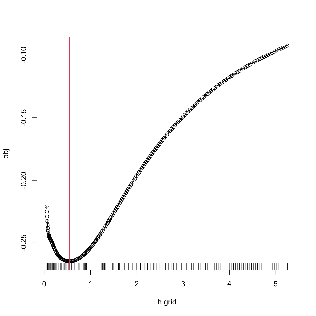
The next cross-validation selector is based on biased cross-validation (BCV). The BCV selector presents a hybrid strategy that combines plug-in and cross-validation ideas. It starts by considering the AMISE expression in (2.17)
\[\begin{align*} \mathrm{AMISE}[\hat f(\cdot;h)]=\frac{1}{4}\mu^2_2(K)R(f'')h^4+\frac{R(K)}{nh} \end{align*}\]
and then plugs-in an estimate for \(R(f'')\) based on a modification of \(R(\hat{f}''(\cdot;h)).\) The modification is
\[\begin{align} \widetilde{R(f'')}:=&\,R(\hat{f}''(\cdot;h))-\frac{R(K'')}{nh^5}\nonumber\\ =&\,\frac{1}{n}\sum_{i=1}^n\sum_{\substack{j=1\\j\neq i}}^n(K_h''*K_h'')(X_i-X_j)\tag{2.21}, \end{align}\]
a leave-out-diagonals estimate of \(R(f'').\) It is designed to reduce the bias of \(R(\hat{f}''(\cdot;h)),\) since \(\mathbb{E}\left[R(\hat{f}''(\cdot;h))\right]=R(f'')+\frac{R(K'')}{nh^5}+O(h^2)\) (Scott and Terrell 1987). Plugging-in (2.21) into the AMISE expression yields the BCV objective function and the BCV bandwidth selector:
\[\begin{align*} \mathrm{BCV}(h)&:=\frac{1}{4}\mu^2_2(K)\widetilde{R(f'')}h^4+\frac{R(K)}{nh},\\ \hat h_\mathrm{BCV}&:=\arg\min_{h>0}\mathrm{BCV}(h). \end{align*}\]
The appealing property of \(\hat h_\mathrm{BCV}\) is that it has a considerably smaller variance compared to \(\hat h_\mathrm{LSCV}.\) This reduction in variance comes at the price of an increased bias, which tends to make \(\hat h_\mathrm{BCV}\) larger than \(h_\mathrm{MISE}.\)
\(\hat h_{\mathrm{BCV}}\) is implemented in R through the function bw.bcv. Again, bw.bcv uses R’s optimize so the bw.bcv.mod function is presented to have better guarantees on finding the adequate minimum.
# Data
set.seed(123456)
x <- rnorm(100)

# BCV gives a warning
bw.bcv(x = x)
## [1] 0.4500924

# Extend search interval
args(bw.bcv)
## function (x, nb = 1000L, lower = 0.1 * hmax, upper = hmax, tol = 0.1 *
##     lower)
## NULL
bw.bcv(x = x, lower = 0.01, upper = 1)
## [1] 0.5070129

# bw.bcv.mod replaces the optimization routine of bw.bcv by an exhaustive search on
# "h.grid" (chosen adaptatively from the sample) and optionally plots the BCV curve
# with "plot.cv"
bw.bcv.mod <- function(x, nb = 1000L,
                       h.grid = diff(range(x)) * (seq(0.1, 1, l = 200))^2,
                       plot.cv = FALSE) {
  if ((n <- length(x)) < 2L)
    stop("need at least 2 data points")
  n <- as.integer(n)
  if (is.na(n))
    stop("invalid length(x)")
  if (!is.numeric(x))
    stop("invalid 'x'")
  nb <- as.integer(nb)
  if (is.na(nb) || nb <= 0L)
    stop("invalid 'nb'")
  storage.mode(x) <- "double"
  hmax <- 1.144 * sqrt(var(x)) * n^(-1/5)
  Z <- .Call(stats:::C_bw_den, nb, x)
  d <- Z[[1L]]
  cnt <- Z[[2L]]
  fbcv <- function(h) .Call(stats:::C_bw_bcv, n, d, cnt, h)
  # h <- optimize(fbcv, c(lower, upper), tol = tol)$minimum
  # if (h < lower + tol | h > upper - tol)
  #   warning("minimum occurred at one end of the range")
  obj <- sapply(h.grid, function(h) fbcv(h))
  h <- h.grid[which.min(obj)]
  if (plot.cv) {
    plot(h.grid, obj, type = "o")
    rug(h.grid)
    abline(v = h, col = 2, lwd = 2)
  }
  h
}

# Compute the bandwidth and plot the BCV curve
bw.bcv.mod(x = x, plot.cv = TRUE)
## [1] 0.5130493

# We can compare with the default bw.bcv output
abline(v = bw.bcv(x = x), col = 3)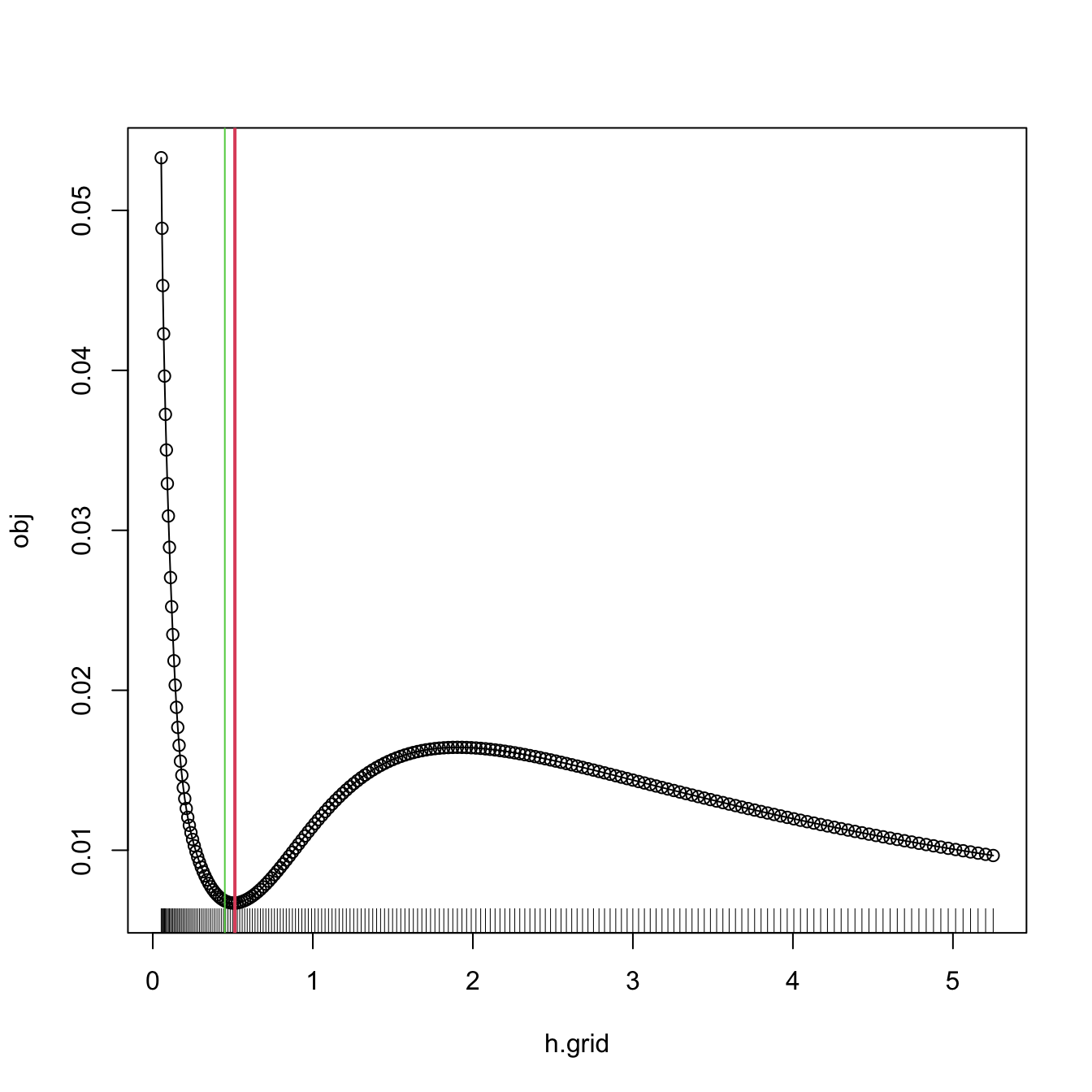
2.4.3 Comparison of bandwidth selectors
We state next some insights from the convergence results of the DPI, LSCV, and BCV selectors. All of them are based in results of the kind
\[\begin{align*} n^\nu(\hat h/h_\mathrm{MISE}-1)\stackrel{d}{\longrightarrow}\mathcal{N}(0,\sigma^2), \end{align*}\]
where \(\sigma^2\) depends only on \(K\) and \(f,\) and measures how variable is the selector. The rate \(n^\nu\) serves to quantify how fast the relative error \(\hat h/h_\mathrm{MISE}-1\) decreases (the larger the \(\nu,\) the faster the convergence). Under certain regularity conditions, we have:
\(n^{1/10}(\hat h_\mathrm{LSCV}/h_\mathrm{MISE}-1)\stackrel{d}{\longrightarrow}\mathcal{N}(0,\sigma_\mathrm{LSCV}^2)\) and \(n^{1/10}(\hat h_\mathrm{BCV}/h_\mathrm{MISE}-1)\stackrel{d}{\longrightarrow}\mathcal{N}(0,\sigma_\mathrm{BCV}^2).\) Both selectors have a slow rate of convergence (compare it with the \(n^{1/2}\) of the CLT). Inspection of the variances of both selectors reveals that, for the normal kernel \(\sigma_\mathrm{LSCV}^2/\sigma_\mathrm{BCV}^2\approx 15.7.\) Therefore, LSCV is considerably more variable than BCV.
\(n^{5/14}(\hat h_\mathrm{DPI}/h_\mathrm{MISE}-1)\stackrel{d}{\longrightarrow}\mathcal{N}(0,\sigma_\mathrm{DPI}^2).\) Thus, the DPI selector has a convergence rate much faster than the cross-validation selectors. There is an appealing explanation for this phenomenon. Recall that \(\hat h_\mathrm{BCV}\) minimizes the slightly modified version of \(\mathrm{BCV}(h)\) given by
\[\begin{align*} \frac{1}{4}\mu_2^2(K)\tilde\psi_4(h)h^4+\frac{R(K)}{nh} \end{align*}\]
and
\[\begin{align*} \tilde\psi_4(h):=&\frac{1}{n(n-1)}\sum_{i=1}^n\sum_{\substack{j=1\\j\neq i}}^n(K_h''*K_h'')(X_i-X_j)\nonumber\\ =&\frac{n}{n-1}\widetilde{R(f'')}. \end{align*}\]
\(\tilde\psi_4\) is a leave-out-diagonals estimate of \(\psi_4.\) Despite being different from \(\hat\psi_4,\) it serves for building a DPI analogous to BCV that points towards the precise fact that drags down the performance of BCV. The modified version of the DPI minimizes
\[\begin{align*} \frac{1}{4}\mu_2^2(K)\tilde\psi_4(g)h^4+\frac{R(K)}{nh}, \end{align*}\]
where \(g\) is independent of \(h.\) The two methods differ on the the way \(g\) is chosen: BCV sets \(g=h\) and the modified DPI looks for the best \(g\) in terms of the \(\mathrm{AMSE}[\tilde\psi_4(g)].\) It can be seen that \(g_\mathrm{AMSE}=O(n^{-2/13}),\) whereas the \(h\) used in BCV is asymptotically \(O(n^{-1/5}).\) This suboptimality on the choice of \(g\) is the reason of the asymptotic deficiency of BCV.
We focus now on exploring the empirical performance of bandwidth selectors. The workhorse for doing that is simulation. A popular collection of simulation scenarios was given by Marron and Wand (1992) and are conveniently available through the package nor1mix. They form a collection of normal \(r\)-mixtures of the form
\[\begin{align*} f(x;\boldsymbol{\mu},\boldsymbol{\sigma},\mathbf{w}):&=\sum_{j=1}^rw_j\phi_{\sigma_j}(x-\mu_j), \end{align*}\]
where \(w_j\geq0,\) \(j=1,\ldots,r\) and \(\sum_{j=1}^rw_j=1.\) Densities of this form are specially attractive since they allow for arbitrarily flexibility and, if the normal kernel is employed, they allow for explicit and exact MISE expressions:
\[\begin{align} \mathrm{MISE}_r[\hat f(\cdot;h)]&=(2\sqrt{\pi}nh)^{-1}+\mathbf{w}'\{(1-n^{-1})\boldsymbol{\Omega}_2-2\boldsymbol{\Omega}_1+\boldsymbol{\Omega}_0\}\mathbf{w},\nonumber\\ (\boldsymbol{\Omega}_a)_{ij}&=\phi_{(ah^2+\sigma_i^2+\sigma_j^2)^{1/2}}(\mu_i-\mu_j),\quad i,j=1,\ldots,r.\tag{2.22} \end{align}\]
# Load package
library(nor1mix)

# Available models
?MarronWand

# Simulating
samp <- rnorMix(n = 500, obj = MW.nm9) # MW object in the second argument
hist(samp, freq = FALSE)

# Density evaluation
x <- seq(-4, 4, length.out = 400)
lines(x, dnorMix(x = x, obj = MW.nm9), col = 2)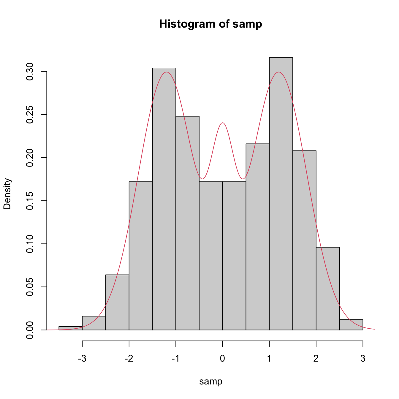
# Plot a MW object directly
# A normal with the same mean and variance is plotted in dashed lines
par(mfrow = c(2, 2))
plot(MW.nm5)
plot(MW.nm7)
plot(MW.nm10)
plot(MW.nm12)
lines(MW.nm10) # Also possible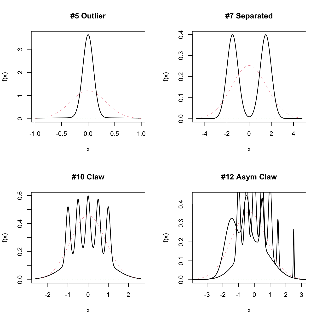
Figure 2.4 presents a visualization of the performance of the kde with different bandwidth selectors, carried out in the family of mixtures of Marron and Wand (1992).
Figure 2.4: Performance comparison of bandwidth selectors. The RT, DPI, LSCV, and BCV are computed for each sample for a normal mixture density. For each sample, computes the ISEs of the selectors and sorts them from best to worst. Changing the scenarios gives insight on the adequacy of each selector to hard- and simple-to-estimate densities. Application also available here.