3.4 Bandwidth selection
Bandwidth selection is, as in kernel density estimation, of key practical importance. Several bandwidth selectors, in the spirit of the plug-in and cross-validation ideas discussed in Section 2.4 have been proposed. There are, for example, a rule-of-thumb analogue (see Section 4.2 in Fan and Gijbels (1996)) and a direct plug-in analogue (see Section 5.8 in Wand and Jones (1995)). For simplicity, we will focus only on the cross-validation bandwidth selector.
Following an analogy with the fit of the linear model, we could look for the bandwidth \(h\) such that it minimizes the RSS of the form
\[\begin{align} \frac{1}{n}\sum_{i=1}^n(Y_i-\hat m(X_i;p,h))^2.\tag{3.24} \end{align}\]
However, this is a bad idea. Attempting to minimize (3.24) always leads to \(h\approx 0\) that results in a useless interpolation of the data. Let’s see an example.
# Grid for representing (3.22)
hGrid <- seq(0.1, 1, l = 200)^2
error <- sapply(hGrid, function(h)
  mean((Y - mNW(x = X, X = X, Y = Y, h = h))^2))

# Error curve
plot(hGrid, error, type = "l")
rug(hGrid)
abline(v = hGrid[which.min(error)], col = 2)
The root of the problem is the comparison of \(Y_i\) with \(\hat m(X_i;p,h),\) since there is nothing that forbids \(h\to0\) and as a consequence \(\hat m(X_i;p,h)\to Y_i.\) We can change this behavior if we compare \(Y_i\) with \(\hat m_{-i}(X_i;p,h),\) the leave-one-out estimate computed without the \(i\)-th datum \((X_i,Y_i)\):
\[\begin{align*} \mathrm{CV}(h)&:=\frac{1}{n}\sum_{i=1}^n(Y_i-\hat m_{-i}(X_i;p,h))^2,\\ h_\mathrm{CV}&:=\arg\min_{h>0}\mathrm{CV}(h). \end{align*}\]
The optimization of the above criterion might seem to be computationally expensive, since it is required to compute \(n\) regressions for a single evaluation of the objective function.
Proposition 3.1 The weights of the leave-one-out estimator \(\hat m_{-i}(x;p,h)=\sum_{\substack{j=1\\j\neq i}}^nW_{-i,j}^p(x)Y_j\) can be obtained from \(\hat m(x;p,h)=\sum_{i=1}^nW_{i}^p(x)Y_i\):
\[\begin{align*} W_{-i,j}^p(x)=\frac{W^p_j(x)}{\sum_{\substack{k=1\\k\neq i}}^nW_k^p(x)}=\frac{W^p_j(x)}{1-W_i^p(x)}. \end{align*}\]
This implies that
\[\begin{align*} \mathrm{CV}(h)=\frac{1}{n}\sum_{i=1}^n\left(\frac{Y_i-\hat m(X_i;p,h)}{1-W_i^p(X_i)}\right)^2. \end{align*}\]
Let’s implement this simple bandwidth selector in R.
# Generate some data to test the implementation
set.seed(12345)
n <- 100
eps <- rnorm(n, sd = 2)
m <- function(x) x^2 + sin(x)
X <- rnorm(n, sd = 1.5)
Y <- m(X) + eps
xGrid <- seq(-10, 10, l = 500)
# Objective function
cvNW <- function(X, Y, h, K = dnorm) {
sum(((Y - mNW(x = X, X = X, Y = Y, h = h, K = K)) /
(1 - K(0) / colSums(K(outer(X, X, "-") / h))))^2)
}
# Find optimum CV bandwidth, with sensible grid
bw.cv.grid <- function(X, Y,
h.grid = diff(range(X)) * (seq(0.1, 1, l = 200))^2,
K = dnorm, plot.cv = FALSE) {
obj <- sapply(h.grid, function(h) cvNW(X = X, Y = Y, h = h, K = K))
h <- h.grid[which.min(obj)]
if (plot.cv) {
plot(h.grid, obj, type = "o")
rug(h.grid)
abline(v = h, col = 2, lwd = 2)
}
h
}
# Bandwidth
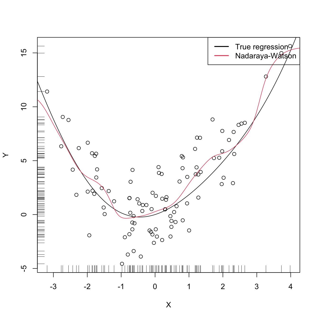
h <- bw.cv.grid(X = X, Y = Y, plot.cv = TRUE)
h
## [1] 0.3117806

# Plot result
plot(X, Y)
rug(X, side = 1); rug(Y, side = 2)
lines(xGrid, m(xGrid), col = 1)
lines(xGrid, mNW(x = xGrid, X = X, Y = Y, h = h), col = 2)
legend("topright", legend = c("True regression", "Nadaraya-Watson"),
       lwd = 2, col = 1:2)