Chapter 12 Differences Between Three or More Things

12.1 Differences Between Things and Differences Within Things

Tufts University (“Tufts”) is an institution of higher learning in the Commonwealth of Massachusetts in the United States of America. Tufts has three campuses: a main campus which covers parts of each of the neighboring cities of Medford, MA and Somerville, MA; a medical center located in Boston, MA; and a veterinary school located in Grafton, MA. Here’s a handy map:

Imagine that somebody asked you – given your access to the map pictured above – to describe the distances between Tufts buildings. What if they asked you if they could comfortably walk or use a wheelchair to get between any two of the buildings? Your answer likely would be that it depends: if one wanted to travel between two buildings that are each on the Medford/Somerville campus, or each on the Boston campus, or each on the Grafton campus, then those distances are small and easily covered without motorized vehicles. If one wanted to travel between campuses, then, yeah, one would need a car or at least a bicycle and probably a bottle of water, too.

We can conceive of the distances between the nine locations marked on the map as if they were just nine unrelated places: some happen to be closer to each other, some happen to be more distant from each other. Or, we can conceive of the distances as a function of campus membership: the distances are small within each campus and the distances are relatively large between campuses. In that conception, there are two sources of variance in the distances: within campus variance and between campus variance, with the former much shorter than the latter. If one were trying to locate a Tufts building, getting the campus correct is much more important than getting the location within each campus correct: if you had an appointment at a building on the Medford/Somerville campus and you went to the wrong Medford/Somerville campus building, there might be time to recover and find the right building; if you went to, say, the Grafton campus, you should probably call, explain, apologize, and try to reschedule.

The example of campus buildings (hopefully) illustrates the basic logic of the Analysis of Variance, more frequently known by the acronym ANOVA. We use ANOVA when there are three or more groups being compared at a time: we could compare pairs of groups using \(t\)-tests, but this would A. inflate the type-I error rate (the more tests you run, the more chances of false alarms),²⁰⁷ and B. fail to give a clear analysis of the omnibus effect of a factor along which all of the groups differ.

As noted in the introduction, ANOVA is based on comparisons of sources of variance. For example, the structure of the simplest ANOVA design – the one-way, between-groups ANOVA – creates a comparison between the variance in the data that comes from between-groups differences and the variance in the data that comes from within-groups differences: if differences in the data that are attributable to the group membership of each datapoint are generally more important than the differences that just occur naturally (and are observable within each group). The logic of ANOVA is represented visually in Figure 12.1 and Figure 12.2. Figure 12.1 is a representation of what happens when the populations of interest are either the same or close to it: there the variance between data points in different groups is the same as the variance between data points within each group, and the is no variance* added by group membership.

Figure 12.1: Visual Representation of ANOVA Logic: No Difference Between Populations

In Figure 12.2, group membership makes a substantial contribution to the overall variance of the data: the variance within each group is the same as in the situation depicted in Figure 12.1, but the differences between the groups slide the populations up and down the \(x\)-axis, spreading out the data as they go.

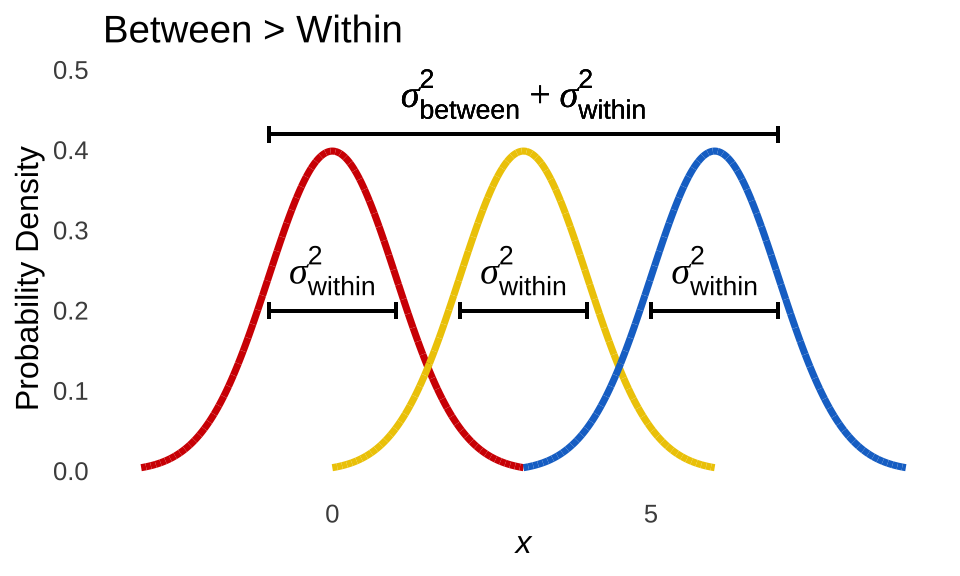
Figure 12.2: Visual Representation of ANOVA Logic: Significant Difference Between Populations

12.1.1 The \(F\)-ratio

The central inference of ANOVA is on the population-level between variance, labeled as \(\sigma^2_{between}\) in Figure 12.1 and Figure 12.2. The null hypothesis for the one-way between-groups ANOVA is:

\[H_0: \sigma^2_{between}=0\] and the alternative hypothesis is:

\[H_1: \sigma^2_{between}>0\] ²⁰⁸The overall variance in the observed data can be decomposed into the sum of the two sources of variance between and within. If the null hypothesis is true and there is no contribution of between-groups differences to the overall variance – which is what is meant by \(\sigma^2_{between}=0\), then all of the variance is attributable to the within-group differences: \(\sigma^2_{between}+\sigma^2_{within}=\sigma^2_{within}\). If, however, the null hypothesis is false and there is any contribution of between-groups difference to the overall variance – \(\sigma^2_{between}>0\), then there will be variance beyond what is attributable to within-groups differences: \(\sigma^2_{between}+\sigma^2_{within}>\sigma^2_{within}\).

Thus, the ANOVA compares \(\sigma^2_{between}+\sigma^2_{within}\) and \(\sigma^2_{within}\). More specifically, it compares \(n\sigma^2_{between}+\sigma^2_{within}\) and \(\sigma^2_{within}\): the influence of \(\sigma^2_{between}\) multiplies with every observation that it impacts (e.g., the influence of between-groups differences cause more variation if there are \(n=30\) observations per group than if there are \(n=3\) observations per group). The way that ANOVA makes this comparison is by evaluating ratios of between-groups variances and within-groups variances: on the population-level, if the ratio is equal to 1, then the two things are the same, if the ratio is greater than one, then the between-groups variance is at least a little bit bigger than 0. Of course, as we’ve seen before with inference, if we estimate that ratio using sample data, any little difference isn’t going to impress us the way a hypothetical population-level little difference would: we’re likely going to need a sample statistic that is comfortably greater than 1.

When we estimate the between-groups plus within-groups variance and within-groups variance using sample data, we calculate what is known as the \(F\)-ratio, also known as the \(F\)-statistic, or just plain \(F\).²⁰⁹The cumulative likelihood of observed \(F\)-ratios are evaluated in terms of the \(F\)-distribution. When we calculate an \(F\)-ratio, we are calculating the ratio between two variances: between variance and within variance. As we know from the chapter on probability distributions, variances are modeled by \(\chi^2\) distributions: \(\chi^2\) distributions comprise the squares of normally-distributed values and given the normality assumption, the numerator of the variance calculation \(\sum(x-\bar{x})^2\) is a normally-distributed set of variables (and dividing by the constant \(n-1\) doesn’t disqualify it). Developed to model the ratio of variances, the \(F\)-distribution is literally the ratio of \(\chi^2\) distributions. The \(F\)-distribution has two sufficient statistics: \(df_{numerator}\) and \(df_{denominator}\), which correspond to the \(df\) of the \(\chi^2\) distribution in the numerator and the \(df\) of the denominator \(\chi^2\) distribution by which it is divided to get the \(F\)-distribution (see illustration in Figure 12.3).

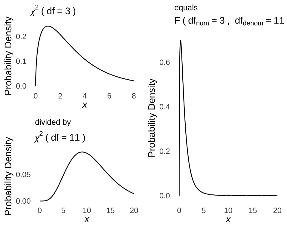
Figure 12.3: Example Derivation of the \(F\)-statistic From a Numerator \(\chi^2\) Distribution with \(df=3\) and a Denominator \(\chi^2\) Distribution with \(df=11\)

The observed \(F\)-ratio is a sample-level estimate of the population-level ratio \(\frac{n\sigma^2_{between}+\sigma^2_{within}}{\sigma^2_{within}}\). If the sample data indicate no difference between the observed variance caused by a combination of between-groups plus within-groups variance and the variance observed within-groups, then \(F\approx 1\) and we will continue to assume \(H_0\). Otherwise, \(F>>1\), and we will reject \(H_0\) in favor of the \(H_1\) that there is some contribution of the differences between groups to the overall variance in the data.

Because of the assumptions involved in constructing the \(F\)-distribution – that at the population-level the residuals are normally distributed and the within-groups variance is the same across groups – the assumptions of normality and homoscedasticity apply to all flavors of ANOVA. For some of those flavors, there will be additional assumptions that we will discuss when we get to them, but normality and homoscedasticity are univerally assumed for classical ANOVAs.

Conceptually, the ANOVA logic applies to all flavors of ANOVA. The tricky part, of course, is how to calculate the \(F\)-ratio, and that will differ across flavors of ANOVA. There are also a number of other features of ANOVA-related analysis that we will discuss, including estimating effect sizes, making more specific between-group comparisons post hoc, a couple of nonparametric alternatives, and the Bayesian counterpart to the classical ANOVA (don’t get too excited: it’s just a “Bayesian ANOVA”). The flavors of ANOVA are more frequently (but less colorfully) described as different ANOVA models or ANOVA designs. We will start our ANOVA journey with the one-way between-groups ANOVA, describing it and its related features before proceeding to more complex models.

Figure 12.4: The features of this ANOVA model include Bluetooth capability, a dishwasher safe detachable stainless steel skirt and disks, cooking notifications, and a 2-year warranty.

12.2 Between-Groups ANOVA models

12.2.1 One-way

12.2.1.1 The Model

To use a one-way between-groups ANOVA is to conceive of dependent-variable scores as being the product of a number of different elements. One is the grand mean \(\mu\), which is the baseline state-of-nature average value in a population. Each number is then also influenced by some condition that causes some numbers to be greater than another. In the case of the one-way between-groups model, the conditions are the levels \(j\) of the factor \(\alpha\)²¹⁰, for example, if the dependent variable is the width of leaves on plants, and the factor \(\alpha\) in question is the amount of time exposed to sunlight and the levels of the factor are 8 hours/day, 10 hours/day, and 12 hours/day, then \(\alpha_1=8\), \(\alpha_2=10\), and \(\alpha_3=12\), and the between-groups difference is the difference caused by the \(j\) different levels of the between-groups factor \(\alpha\). The last element is the within-groups variance, which falls into the more general categories of error or residuals. It is the naturally-occurring variation within each condition. To continue the example of the plants and the sunlight: not every plant that is exposed to the same sunlight for the same duration will have leaves that are exactly the same width. In this model, the within-groups influence is symbolized by \(\epsilon_{ij}\), indicating that the error (\(\epsilon\)) exists within each individual observation (\(i\)) and at each level of the treatment (\(j\)).

In a between-groups design, each observation comes from an independent group, that is, each observation comes from one and only one level of the treatment.

Could we account for at least some of the within-groups variation by identifying individual differences? Sure, and that’s the point of within-groups designs, but it’s not possible unless we observe each plant under different sunlight Conditions, which is not part of a between-groups design. For more on when we want to (or have to) use between-groups designs instead of within-groups designs, please refer to the chapter on differences between two things.

Thus, each value \(y\) of the dependent variable is said to be determined by the sum of the grand mean \(\mu\), the mean of the factor-level \(\alpha_j\), and the individual contribution of error \(\epsilon_{ij}\); and because \(y\) is influenced by factor level and treatment, it gets the subscript \(ij\):

\[y_{ij}=\mu+\alpha_j+\epsilon_i\] If you think that equation vaguely resembles a regression model, that’s because it is:

ANOVA is a special case of multiple regression where there is equal \(n\) per factor-level.

ANOVA is regression-based much as the \(t\)-test can be expressed as a regression analysis. In fact, while we are making connections, the \(t\)-test is a special case of ANOVA. If, for example, you enter data with two levels of a between-groups factor, you will get precisely the same results – with an \(F\) statistic instead of a \(t\) statistic – as you would for an independent-groups \(t\)-test.²¹¹

12.2.1.2 The ANOVA table

The results of ANOVA can be represented by an ANOVA table. The standard ANOVA table includes the following elements:

1. Source (or Source of Variance, or SV): the leftmost column represents the decomposition of the elements that influence values of the dependent variable (except the grand mean \(\mu\)). For the one-way between-groups ANOVA, the listed sources are typically between groups (or just between) and within groups (or just within), with an entry for total variance often included. To increase the generality of the table – which will be helpful because we are about to talk about a whole bunch of ANOVA tables, we, we can call the between variance \(A\) to indicate that it is the variance associated with factor \(A\) and we can call the within variance the error.

2. Degrees of Freedom (\(df\)): the degrees of freedom associated with each source. These are the degrees of freedom that are associated with the variance calculation (i.e., the variance denominator) for each source of variance.

3. Sums of Squares (\(SS\)): The numerator of the calculation for the variance (\(\sum(x-\bar{x})^2\)) associated with each source.

4. Mean Squares (\(MS\)): The estimate of the variance for each source. It is equal to the ratio of \(SS\) and \(df\) that are respectively associated with each source. Note: \(MS\) are not calculated for the total because there is no reason whatsoever to care about the total \(MS\).

5. \(F\): The \(F\)-ratio. The \(F\)-ratio is the test statistic for the ANOVA. For the one-way between-groups design (and also for the one-way within-groups design but we’ll get to that later), there is only one \(F\)-ratio, and it is the ratio of the between-groups \(MS\) (\(MS_{A}\)) to within-groups \(MS\) \(MS_e\).

In addition to the five columns described above, there is a sixth column that is extremely optional to include:

6. Expected Mean Squares (\(EMS\)): a purely algebraic, non-numeric representation of the population-level variances associated with each source. As noted earlier, the population-level comparison represented with sample data by the \(F\)-statistic is \(\frac{n\sigma^2_{between}+\sigma^2_{within}}{\sigma^2_{within}}\), which can somewhat more simply be annotated \(\frac{n\sigma^2_\alpha+\sigma^2_\epsilon}{\sigma^2_\epsilon}\). In other words, it is the ratio of the sum of between-groups variance – which is multiplied by the number of observations per group – plus the within-groups variance divided by the within-groups variance. The \(EMS\) for each group lists the terms that are represented by each source. For between-groups variance – or factor \(\alpha\) – the \(EMS\) is the numerator of the population-level \(F\)-ratio \(n\sigma^2_\alpha+\sigma^2_\epsilon\). For the within-groups variance – or the error (\(\epsilon\)) – it is \(\sigma^2_\epsilon\). The \(EMS\) are helpful for two things: keeping track of how to calculate the \(F\)-ratio for a particular factor in a particular ANOVA model (admittedly, this isn’t really an issue for the one-way between-groups ANOVA since there is only one way to calculate an \(F\)-statistic and it’s relatively easy to remember it), and calculating the effect-size statistic \(\omega^2\). Both of those things can be accomplished without explicitly knowing the \(EMS\) for each source of variance, which is why the \(EMS\) column of the ANOVA table is eminently skippable (but, if you do need to include it – presumably at the behest of some evil stats professor – please keep in mind that there are no numbers to be calculated for \(EMS\): they are strictly algebraic formulae).

Here is the ANOVA table – with \(EMS\) – for the one-way between-groups ANOVA model with formula guides for how to calculate the values that go in each cell:

\(SV\)	\(df\)	\(SS\)	\(MS\)	\(F\)	\(EMS\)
\(A\)	\(j-1\)	\(n\sum(y_{\bullet j}-y_{\bullet\bullet})^2\)	\(SS_A/df_A\)	\(MS_A/MS_e\)	\(n\sigma^2_\alpha+\sigma^2_\epsilon\)
\(Error\)	\(n-1\)	\(\sum(y_{ij}-y_{\bullet j})^2\)	\(SS_A/df_e\)		\(\sigma^2_\epsilon\)
\(Total\)	\(jn-1\)	\(\sum(y_{ij}-y_{\bullet\bullet})^2\)

In the table above, the bullet (\(\bullet\)) replaces the subscript \(i\), \(j\), or both to indicate that the \(y\) values are averaged across each level of the subscript being replaced. \(y_{\bullet j}\) indicates the average of all of the \(y\) values in each \(j\) averaged across all \(i\) observations and \(y_{\bullet \bullet}\) is the grand mean of all of the \(y\) values averaged across all \(i\) observations in each of \(j\) Conditions. Thus, \(SS_A\) is equal to the sum of the squared differences between each group mean \(y_{\bullet j}\) and the grand mean \(y_{\bullet \bullet}\) times the number of observations in each group \(n\), \(SS_e\) is equal to the sum of the sums of the squared differences between each observation \(y_{ij}\) and the mean \(y_{\bullet j}\) of the group to which it belongs, and \(SS_total\) is equal to the sum of the squared differences between each observation \(y_{ij}\) and the grand mean \(y_{\bullet \bullet}\).

In the context of ANOVA, \(n\) always refers to the number of observations per group. If one needs to refer to all of the observations (e.g. all the participants in an experiment that uses ANOVA to analyze the data), \(N\) is preferred to (hopefully) avoid confusion. In the classic ANOVA design, \(n\) is always the same between all groups: if \(n\) is not the same between groups, then technically the analysis is not an ANOVA. That’s not a dealbreaker for statistical analysis, though: if \(n\) is unequal between groups, the data can be analyzed in a regression context with the general linear model and the procedure will return output that is pretty-much-identical to the ANOVA table. The handling of unequal \(n\) is beyond the scope of this course, but I assure you, it’s not that bad, and you’ll probably get to it next semester.

12.2.1.3 Example

Please imagine that the following data are observed in a between-groups design:

Condition 1	Condition 2	Condition 3	Condition 4
-3.10	7.28	0.12	8.18
0.18	3.06	5.51	9.05
-0.72	4.74	5.72	11.21
0.09	5.29	5.93	7.31
-1.66	7.88	6.56	8.83
Grand Mean = 4.57

12.2.1.3.0.1 Calculating \(df\)

There are \(j=4\) levels of factor \(\alpha\), thus, \(df_A=j-1=3\). There are \(n=5\) observations in each group, so \(df_e=j(n-1)=4(4)=16\). The total \(df_{total}=jn-1=(4)(5)-1=19\). Note that \(df_A+df_e=df_{total}\), and that \(df_{total}=N-1\) (or the total number of observations minus 1). Both of those facts will be good ways to check your \(df\) math as models become more complex.

12.2.1.3.0.2 Calculating \(SS_A\)

\(SS_A\) is the sum of squared deviations between the level means and the grand mean multiplied by the number of observations in each level. Another way of saying that is that for each observation, we take the mean of the level to which that observation belongs, subtract the grand mean, square the difference, and sum all of those squared differences. Because \(n\) is the same across groups by the ANOVA definition, it is no difference to multiply the squared differences between the group means and the grand mean by \(n\) or to add up the squared differences between the group means for every observation; I happen to find the latter more visually convincing for pedagogical purposes, as in the table below:

Condition 1	\((y_{\bullet 1}-y_{\bullet \bullet})^2\)	Condition 2	\((y_{\bullet 2}-y_{\bullet \bullet})^2\)	Condition 3	\((y_{\bullet 3}-y_{\bullet \bullet})^2\)	Condition 4	\((y_{\bullet 4}-y_{\bullet \bullet})^2\)
-3.10	31.49	7.28	1.17	0.12	0.04	8.18	18.89
0.18	31.49	3.06	1.17	5.51	0.04	9.05	18.89
-0.72	31.49	4.74	1.17	5.72	0.04	11.21	18.89
0.09	31.49	5.29	1.17	5.93	0.04	7.31	18.89
-1.66	31.49	7.88	1.17	6.56	0.04	8.83	18.89

The sum of the values in the shaded columns is 257.94: that is the value of \(SS_A\).

12.2.1.3.0.3 Calculating \(SS_e\)

The \(SS_e\) for this model – or, the within-groups variance – is the sum across levels of factor \(A\) of the sums of the squared differences between each \(y_ij\) value of the dependent variable and the mean \(y_{\bullet j}\) of the level to which it belongs:

Condition 1	\((y_{i1}-y_{\bullet j})^2\)	Condition 2	\((y_{i 2}-y_{\bullet j})^2\)	Condition 3	\((y_{i 3}-y_{\bullet j})^2\)	Condition 4	\((y_{i 4}-y_{\bullet j})^2\)
-3.10	4.24	7.28	2.66	0.12	21.60	8.18	0.54
0.18	1.49	3.06	6.71	5.51	0.55	9.05	0.02
-0.72	0.10	4.74	0.83	5.72	0.91	11.21	5.26
0.09	1.28	5.29	0.13	5.93	1.35	7.31	2.58
-1.66	0.38	7.88	4.97	6.56	3.21	8.83	0.01

The sum of the values in the shaded columns is 58.82: that is \(SS_e\).

12.2.1.3.0.4 Calculating \(SS_{total}\)

\(SS_{total}\) is the total sums of squares of the dependent variable \(y\):

\[\sum_{i=1}^N(y_{ij}-y_{\bullet \bullet})^2\] To calculate \(SS_{total}\), we sum the squared differences between each observed value \(y_{ij}\) and the grand mean \(y_{\bullet \bullet}\):

Condition 1	\((y_{i1}-y_{\bullet \bullet})^2\)	Condition 2	\((y_{i 2}-y_{\bullet \bullet})^2\)	Condition 3	\((y_{i 3}-y_{\bullet \bullet})^2\)	Condition 4	\((y_{i 4}-y_{\bullet \bullet})^2\)
-3.10	58.83	7.28	7.34	0.12	19.80	8.18	13.03
0.18	19.27	3.06	2.28	5.51	0.88	9.05	20.07
-0.72	27.98	4.74	0.03	5.72	1.32	11.21	44.09
0.09	20.07	5.29	0.52	5.93	1.85	7.31	7.51
-1.66	38.81	7.88	10.96	6.56	3.96	8.83	18.15

The sum of the shaded values is 316.76, which is \(SS_{total}\). It is also equal to \(SS_A\)+\(SS_e\), which is important for two reasons:

1. It means we did the math right, and

2. The total sums of squares of the dependent variable is completely broken down by the sums of squares associated with the between-groups factor and the sums of squares associated with within-groups variation, with no overlap between the two. The fact that the total variation is exactly equal to the sum of the variation contributed by the two sources demonstrates the principle of orthogonality: where two or more factors do not account for the same variance because they are uncorrelated with each other.

Orthogonality is an important statistical concept that shows up in multiple applications, including one of the post hoc tests to be discussed below and, critically, all ANOVA models. In every ANOVA model, the variance contributed to the dependent variable will be broken down orthogonally between each of the sources, meaning that \(SS_{total}\) will always be precisely equal to the sum of the \(SS\) for all sources of variance for each model.

12.2.1.3.0.5 Calculating \(MS_A\), \(MS_B\), and \(F\)

As noted in the ANOVA table above, the mean squares for each source of variance is the ratio of the sums of squares associated with that source divided by the degrees of freedom for that source. For the example data:

\[MS_A=\frac{SS_A}{df_A}=\frac{257.94}{3}=85.98\] \[MS_e=\frac{SS_e}{df_e}=\frac{58.82}{16}=3.68\]

The observed \(F\)-ratio is the ratio of the \(MS_A\) to \(MS_e\), and is annotated with the degrees of freedom associated with the numerator of that ratio \(df_{numerator}\) (usually abbreviated \(df_{num}\)) and degrees of freedom associated with the denominator of that ratio \(df_{denominator}\) (usually abbreviated \(df_{denom}\)) in parenthesis following the letter \(F\):

\[F(3, 16)=\frac{MS_A}{MS_e}=\frac{85.98}{3.68}=23.39\]

12.2.1.3.0.6 There is nothing to calculate for \(EMS\)

The EMS for this model are simply \(n\sigma^2_\alpha + \sigma^2_\epsilon\) for factor \(A\) and \(\sigma^2_\epsilon\) for the error.

Now we are ready to fill in our ANOVA table.

12.2.1.3.0.7 Example ANOVA Table and Statistical Inference

Here is the ANOVA table for the example data:

\(SV\)	\(df\)	\(SS\)	\(MS\)	\(F\)	\(EMS\)
\(A\)	3	257.94	85.98	23.39	\(n\sigma^2_\alpha+\sigma^2_\epsilon\)
\(Error\)	16	58.82	3.68		\(\sigma^2_\epsilon\)
\(Total\)	19	316.76

The \(F\)-ratio is evaluated in the context of the \(F\)-distribution associated with the observed \(df_{num}\) and \(df_{denom}\). For our example data, the \(F\)-ratio is 23.39: the cumulative likelihood of observing an \(F\)-statistic of 23.39 or greater given \(df_{num}=3\) and \(df_{denom}=16\) – the area under the \(F\)-distribution curve with those specific parameters at or beyond 23.39, is:

pf(23.39, df1=3, df2=16, lower.tail=FALSE)

## [1] 4.30986e-06

Since \(4.3\times 10^-6\) is smaller than any reasonable value of \(\alpha\), we will reject the null hypothesis that \(\sigma^2_\alpha=0\) in favor of the alternative hypothesis that \(\sigma^2_\alpha>0\): there is a significant effect of the between-groups factor.

12.2.1.3.0.8 ANOVA in R

There are several packages to calculate ANOVA results in R, but for most purposes, the base command aov() will do. The aov() command returns an object that can then be summarized with the summary() command wrapper to give the elements of the traditional ANOVA table.

aov() expects a formula and data structure similar to what we used for linear regression models and for tests of homoscedasticity. Thus, it is best to put the data into long format. Using the example data from above:

DV<-c(Condition1, Condition2, Condition3, Condition4)
Factor.A<-c(rep("Condition 1", length(Condition1)),
            rep("Condition 2", length(Condition2)),
            rep("Condition 3", length(Condition3)),
            rep("Condition 4", length(Condition4)))

one.way.between.groups.example.df<-data.frame(DV, Factor.A)

summary(aov(DV~Factor.A,
            data=one.way.between.groups.example.df))

##             Df Sum Sq Mean Sq F value   Pr(>F)    
## Factor.A     3 257.94   85.98   23.39 4.31e-06 ***
## Residuals   16  58.82    3.68                     
## ---
## Signif. codes:  0 '***' 0.001 '**' 0.01 '*' 0.05 '.' 0.1 ' ' 1

12.2.2 Effect Size Statistics

The effect-size statistics for ANOVA models are based on the same principle as \(R^2\): they are measures of the proportion of the overall variance data that is explained by the factor(s) in the model (as opposed to the error). In fact, one ANOVA-based effect-size statistic – \(\eta^2\) – is precisely equal to \(R^2\) for the one-way between-groups model (remember: ANOVA is a special case of multiple regression). Since they are proportions, the ANOVA-based effect-size statistics range from 0 to 1, with larger values indicating increased predictive power for the factor(s) in the model relative to the error.

We here will discuss two ANOVA-based effect-size statistics: \(\eta^2\) and \(\omega^2\).²¹² Estimates of \(\eta^2\) and of \(\omega^2\) tend to be extremely close: if you calculate both statistics for the same data, you are less likely to observe that the two statistics disagree as to the general size of an effect than you are to see them be separated by a couple percent, or tenths of a percent, or hundredths of a percent.

Of \(\eta^2\) and \(\omega^2\), \(\eta^2\) is vastly easier to calculate, and as noted just above, not far off from estimates of \(\omega^2\) for the same data. \(\eta^2\) is also more widely used and understood. The only disadvantage is that \(\eta^2\) is a biased estimator of effect size: it’s consistently too big (one can test that with Monte Carlo simulations and/or synthetic data – using things like the rnorm() command in R – to check the relationship between the magnitude of a statistical estimate and what it should be given that the underlying distribution characteristics are known). That bias is usually more pronounced for smaller sample sizes: if you google “eta squared disadvantage,” the first few results will be about the estimation bias of \(\eta^2\) and the problems it has with relatively small \(n\). Again, it’s not a gamechanging error, but if you are pitching your results to an audience of ANOVA-based effect-size purists, they may be looking for you to use the unbiased estimator \(\omega^2\).

In addition to being unbiased, the other advantage that \(\omega^2\) has is that it is equivalent to the statistic known as the intraclass correlation (ICC), which is usually considered a measure of the psychometric construct reliability. ANOVA-based effect size statistics – including both \(\eta^2\) and \(\omega^2\) – can also be interpreted as measuring reliability of a measure: if a factor or factors being measured make a big difference in the scores, then assessing dependent variables based on those factors should return reliable results over time. In the world of psychometrics – which I can tell you from lived experience is exactly as exciting and glamorous as it sounds – some analysts report ICC statistics and some report \(\omega^2\) statistics and a suprisingly large proportion don’t know that they are talking about the same thing.

12.2.2.1 Calculating \(\eta^2\)

For the one-way between-groups ANOVA model, \(\eta^2\) is a ratio of sums of squares: the sums of squares associated with the factor \(SS_A\) to the total sums of squares \(SS_{total}\). It is thus the proportion of observed sample-level variance associated with the factor:

\[\eta^2=\frac{SS_A}{SS_{total}}\] For the example data, the observed \(\eta^2\) is:

\[\eta^2=\frac{SS_A}{SS_{total}}=\frac{257.94}{316.76}=0.81\] which is a large effect (see the guidelines for interpreting ANOVA-based effect sizes below).

12.2.2.2 Calculating \(\omega^2\)

The \(\omega^2\) statistic is an estimate of the population-level variance that is explained by the factor(s) in a model relative to the population-level error.²¹³ The theoretical population-level variances are known as population variance components: for the one-way between-groups ANOVA model, the two components are the variance from the independent-factor variable \(\sigma^2_\alpha\) and the variance associated with error \(\sigma^2_\epsilon\).

As noted above, the between-groups variance in the one-way model is classified as \(n\sigma^2_\alpha + \sigma^2_\epsilon\), and is estimated in the sample data by \(MS_A\); the within-groups variance is classified as \(\sigma^2_\epsilon\), and is estiamted in the sample data by \(MS_e\): these are the terms listed for factor A and for the error, respectively, in the \(EMS\) of the ANOVA table.

\(\omega^2\) is the ratio of the population variance component for factor A \(\sigma^2_\alpha\) divided by the sum of the population variance components \(\sigma^2_\alpha +\sigma^2_\epsilon\):

\[\omega^2=\frac{\sigma^2_\alpha}{\sigma^2_\alpha + \sigma^2_\epsilon}\]

As noted above, \(MS_e\) is an estimator of \(\sigma^2_\epsilon\) (\(\sigma^2_\epsilon\) gets a hat because it’s an estimate):

\[\hat{\sigma}^2_\epsilon=MS_e\]

That takes care of one population variance component. \(MS_A\) is an estimator of \(n\sigma^2_\alpha + \epsilon\): if we subtract \(MS_e\) (being the estimate of \(\sigma^2_\epsilon\)) from \(MS_A\) and divide by \(n\), we get the population variance component \(\sigma^2_\alpha\):

\[\hat{\sigma}^2_\alpha=\frac{MS_A-MS_e}{n}\] Please note that a simpler and probably more meaningful way to conceive of \(\sigma^2_\alpha\) is that it is literally the variance of the condition means. For the one-way between-groups ANOVA model, it is more straightforward to simply calculate the variance of the condition means than to use the above formula, but it gets moderately more tricky to apply that concept to more complex designs.

We’re not quite done with \(\hat{\sigma}^2_\alpha\) yet: there is one more consideration.

12.2.2.2.1 Random vs. Fixed Effects

The value of \(\hat{\sigma}^2_\alpha\) as calculated above has for its denominator \(df_A\), which is \(j-1\). Please recall that the formula for a sample variance – \(s^2=\frac{\sum(x-\bar{x})^2}{n-1}\) also has an \(x-1\) term in the denominator. In the case of a sample variance, that’s an indicator that the variance refers to a sample that is much smaller than the population from which it comes. In the case of a population variance component, that indicates that the number of levels \(j\) of the independent-variable factor \(A\) is a sample of levels much smaller than the total number of possible levels of the factor. When the number of levels of the independent variable represent just some of the possible levels of the independent variable, that IV is known as a random-effects factor (the word “random” may be misleading: it doesn’t mean that factors were chosen out of a hat or via a random number generator, just that there are many more possible levels that could have been tested). For example, a health sciences researcher might be interested in the effect of different U.S. hospitals on health outcomes. They may not be able to include every hospital in the United States in the study, but rather 3 or 4 hospitals that are willing to participate in the study: in that case, hospital would be a random effect with those 3 or 4 levels (and the within-groups variable would be the patients in the hospitals).

A fixed-effect factor is one in which all (or, technically, very nearly all) possible levels of the independent variables are examined. To recycle the example of studying the effect of hospitals on patient outcomes, we might imagine that instead of hospitals in the United States, the independent variable of interest were hospitals in one particular city, in which case 3 or 4 levels might represent all possible levels of the variable. Please note that it is not the absolute quantity of levels that determines whether an effect is random or fixed but the relative quantity of observed levels to the total possible set of levels of interest.

When factor A is fixed, we have to replace the denominator \(j-1\) with \(j\) (to indicate that the variance is a measure of all of the levels of interest of the IV). We can do that pretty easily by multiplying the population variance component \(\hat{\sigma}^2_\alpha\) by \(j-1\) – which is equal to \(df_A\) – and then dividing the result by \(j\) – which is equal to \(df_A+1\). We can accomplish that more simply by multiplying the estimate of \(\sigma^2_\alpha\) by the term \(\frac{df_A}{df_A+1}\).

So, for random effects in terms of Expected Mean Squares:

\[\hat{\sigma}^2_\alpha=\frac{MS_A-MS_e}{n}\] \(\sigma^2_\alpha\), as noted above, is the variance of the means of the levels of factor \(A\). If factor \(A\) is random, then \(\sigma^2_\alpha\) is, specifically, the sample variance of the means of the levels of factor \(A\) about the grand mean \(y_{\bullet \bullet}\):

\[\hat{\sigma}^2_\alpha=\frac{\sum(y_{\bullet j}-y_{\bullet \bullet})^2}{j-1}\]

and for fixed effects:

\[\hat{\sigma}^2_\alpha=\frac{MS_A-MS_e}{n}\left[\frac{df_A}{df_A+1}\right]\]

which is equivalent to the population variance of the means of the levels of factor \(A\) about the grand mean \(y_{\bullet \bullet}\):

\[\hat{\sigma}^2_\alpha=\frac{\sum(y_{\bullet j}-y_{\bullet \bullet})^2}{j}\]

One more note on population variance components before we proceed to calculating \(\omega^2\) for the sample data: the fact that the numerator of \(\hat{\sigma}^2_x\) (using \(x\) as a generic indicator of a factor that can be \(\alpha\), \(\beta\), \(\gamma\), etc. for more complex models) includes a subtraction term (in the above equation, it’s \(MS_a-MS_e\)), it is possible to end up with a negative estimate for \(\hat{\sigma}^2_x\) if the \(F\)-ratio for that factor is not significant. This really isn’t an issue for the one-way between-groups ANOVA design because if \(F_A\) is not significant then there is no effect to report and, as noted in the chapter on differences between two things, we do not report effect sizes when effects are not significant. But, it can happen for population variance components in factorial designs. If that is the case, we set all negative population variance components to 0.

Using the example data, assuming that factor A is a random effect:

\[\hat{\sigma}^2_\epsilon=MS_e=3.68\] \[\hat{\sigma}^2_\alpha=\frac{MS_A-MS_e}{n}=\frac{85.98-3.68}{5}=16.46\] and:

\[\omega^2=\frac{\hat{\sigma}^2_\alpha}{\hat{\sigma}^2_\alpha + \hat{\sigma}^2_\epsilon}=\frac{16.46}{16.46+3.68}=0.82\] Assuming that factor A is a fixed effect:

\[\hat{\sigma}^2_\epsilon=MS_e=3.68\]

\[\hat{\sigma}^2_\alpha=\frac{MS_A-MS_e}{n}\left[\frac{df_A}{df_A+1}\right]=\frac{85.98-3.68}{5}\left(\frac{3}{4}\right)=12.35\] and:

\[\omega^2=\frac{\hat{\sigma}^2_\alpha}{\hat{\sigma}^2_\alpha + \hat{\sigma}^2_\epsilon}=\frac{12.35}{12.35+3.68}=0.77\]

12.2.2.3 Effect-size Guidelines for \(\eta^2\) and \(\omega^2\)

As is the case for most classical effect-size guidelines, Cohen (2013) provided interpretations for \(\eta^2\) and \(\omega^2\). In his book Statistical Power Analysis for the Behavioral Sciences – which is the source for all of Cohen’s effect-size guidelines – Cohen claims that \(\eta^2\) and \(\omega^2\) are measures of the same thing (which is sort of true but also sort of not) and thus should have the same guidelines for what effects are small, medium, and large (which more-or-less works out because \(\eta^2\) and \(\omega^2\) are usually so similar in magnitude):

\(\eta^2\) or \(\omega^2\)	Interpretation
\(0.01\to 0.6\)	Small
\(0.6 \to 0.14\)	Medium
\(0.14\to 1\)	Large

Thus, the \(\eta^2\) value and the \(\omega^2\) values assuming either random or fixed effects for the sample data all fall comfortably into the large effect range.²¹⁴

12.2.3 Post hoc tests

Roughly translated, post hoc is Latin for after this. Post hoc tests are conducted after a significant effect of a factor has been established to learn more about the nature of an effect, i.e.: which levels of the factor are associated with higher or lower scores?

Post hoc tests can help tell the story of data beyond just a significant \(F\)-ratio in several ways. There is a test that compares experimental conditions to a single control condition (the Dunnett common control procedure). There are tests that compare the average(s) of one set of conditions to the average(s) of another set of conditions (including orthogonal contrasts and Scheffé contrasts). There are also post hoc tests that compare the differences between each possible pair of condition means (including Dunn-Bonferroni tests, Tukey’s HSD, and the Hayter-Fisher test). The choice of post hoc test depends on the story you are trying to tell with the data

12.2.3.1 Pairwise Comparisons

12.2.3.1.1 Dunn-Bonferroni Tests

The use of Dunn-Bonferroni tests, also known as applying the Dunn-Bonferroni correction, is a catch-all term for any kind of statistical procedure where multiple hypotheses are conducted simultaneously and the type-I error rate is reduced for each test of hypotheses in order to avoid inflating the overall type-I error rate. For example, a researcher testing eight different simple regression models using eight independent variables to separately predict the dependent variable – that is, running eight different regression commands – might compare the p-values associated each of the eight models to an \(\alpha\) that is \(1/8th\) the size of the overall desired \(\alpha\)-rate (otherwise, she would risk committing eight times the type-I errors she would with a single model).

In the specific context of post hoc tests, the Dunn-Bonferroni test is an independent-samples t-test for each of the condition means. The only difference is that one takes the \(\alpha\)-rate of one’s preference – say, \(\alpha=0.05\), and divides it by the number of possible multiple comparisons that can be performed on the condition means:

\[\alpha_{Dunn-Bonferroni}=\frac{\alpha_{overall}}{\#~of~pairwise~comparisons}\]

(it may be tempting to divide the overall \(\alpha\) by the number of comparisons performed instead of the number possible, but then one could just run one comparison with regular \(\alpha\) and thus defeat the purpose)

To use the example data from above, let’s imagine that we are interested in applying the Dunn-Bonferroni correction to a post hoc comparison of the mean of Condition 1 and Condition 2. To do so, we simply follow the same procedure as for the independent-samples t-test and adjust the \(\alpha\)-rate. Assuming we start with \(\alpha=0.05\), since there are 4 groups in the data, there are \(_4C_2=6\) possible pairwise comparisons, so the Dunn-Bonferroni-adjusted \(\alpha\)-rate is \(0.05/6=0.0083\)

t.test(Condition1, Condition2, paired=FALSE)

## 
##  Welch Two Sample t-test
## 
## data:  Condition1 and Condition2
## t = -6.2688, df = 7.1613, p-value = 0.0003798
## alternative hypothesis: true difference in means is not equal to 0
## 95 percent confidence interval:
##  -9.204768 -4.179232
## sample estimates:
## mean of x mean of y 
##    -1.042     5.650

The observed \(p\)-value of \(0.0002408<0.0125\), so we can say that there is a signficant difference between the groups after applying the Dunn-Bonferroni correction.

Please also note that if you need to for any reason, you could also multiply the observed \(p\)-value by the number of possible pairwise comparisons and compare the result to the original \(\alpha\). It works out to be the same thing, a fact that is exploited by the base R command pairwise.t.test(), in which you can use the p.adjust="bonferroni"²¹⁵ to conduct pairwise Dunn-Bonferroni tests on all of the conditions in a set simultaneously:

DV<-c(Condition1, Condition2, Condition3, Condition4)
Factor.A<-c(rep("Condition 1", length(Condition1)),
            rep("Condition 2", length(Condition2)),
            rep("Condition 3", length(Condition3)),
            rep("Condition 4", length(Condition4)))

pairwise.t.test(DV, Factor.A, p.adjust="bonferroni", pool.sd = FALSE, paired=FALSE)

## 
##  Pairwise comparisons using t tests with non-pooled SD 
## 
## data:  DV and Factor.A 
## 
##             Condition 1 Condition 2 Condition 3
## Condition 2 0.0023      -           -          
## Condition 3 0.0276      1.0000      -          
## Condition 4 2.3e-05     0.1125      0.1222     
## 
## P value adjustment method: bonferroni

12.2.3.1.2 Tukey’s HSD

Tukey’s Honestly Significant Difference (HSD) Test is a way of determining whether the difference between two condition means is (honestly) significant. The test statistic for Tukey’s HSD test is the studentized range statistic \(q\), where for two means \(y_{\bullet1}\) and \(y_{\bullet2}\):

\[q=\frac{y_{\bullet1}-y_{\bullet2}}{\sqrt{\frac{MS_e}{n}}}\] ^[In this chapter, we are dealing exclusively with classical ANOVA models with equal \(n\) per group. The \(q\) statistic for the HSD test can also handle cases of unequal \(n\) for post hoc tests of results from generalized linear models by using the denominator:

\[\sqrt{\frac{MS_e}{2}\left(\frac{1}{n_1}+\frac{1}{n_2}\right)}\] which is known as the Kramer correction. If using the Kramer correction, the more appropriate name for the test is not the Tukey test but rather the Tukey-Kramer procedure.]

The critical value of \(q\) depends on the number of conditions and on \(df_e\): those values can be found in tables such as this one.

For any given pair of means, the observed value of \(q\) is given by the difference between those means divided by \(\sqrt{MS_e/n}\), where \(MS_e\) comes from the ANOVA table and \(n\) is the number in each group: if the observed \(q\) exceeds the critical \(q\), then the difference between those means is honestly significantly different.

When performing the Tukey HSD test by hand, it also can be helpful to start with the critical \(q\) and calculate a critical HSD value such that any observed difference between means that exceeds the critical HSD is itself honestly significant:

\[HSD_{crit}=q_{crit}\sqrt{\frac{MS_e}{n}}\]

But, it is unlikely that you will be calculating HSDs by hand. The base R command TukeyHSD() wraps an aov() object – in the same way that we can wrap summary() around an aov() object to get a full-ish ANOVA table – and returns results about the differences between means with confidence intervals and \(p\)-values:

TukeyHSD(aov(DV~Factor.A,
            data=one.way.between.groups.example.df))

##   Tukey multiple comparisons of means
##     95% family-wise confidence level
## 
## Fit: aov(formula = DV ~ Factor.A, data = one.way.between.groups.example.df)
## 
## $Factor.A
##                           diff        lwr       upr     p adj
## Condition 2-Condition 1  6.692  3.2225407 10.161459 0.0002473
## Condition 3-Condition 1  5.810  2.3405407  9.279459 0.0010334
## Condition 4-Condition 1  9.958  6.4885407 13.427459 0.0000022
## Condition 3-Condition 2 -0.882 -4.3514593  2.587459 0.8847332
## Condition 4-Condition 2  3.266 -0.2034593  6.735459 0.0687136
## Condition 4-Condition 3  4.148  0.6785407  7.617459 0.0165968

According to the results here, there are honestly significant differences (assuming \(\alpha=0.05\)) between Condition 2 and Condition 1, between Condition 3 and Condition 1, between Condition 4 and Condition 1, and between Condition 4 and Condition 3. All other differences between level means are not honestly significant.

12.2.3.1.3 Hayter-Fisher Test

The Hayter-Fisher test is identical to the Tukey HSD, but with a smaller critical \(q\) value, which makes this test more powerful than the Tukey HSD test. The critical value of \(q\) used for the Hayter-Fisher test is the value listed in tables for \(k-1\) groups given the same \(df_e\) (in the table linked above, it is the critical \(q\) listed one column immediately to the left of the value one would use for Tukey’s HSD).

The condition that comes from being able to use a smaller critical \(q\) value is that the Hayter-Fisher test can only be used following significant \(F\) test. However, since you shouldn’t be reporting results of post hoc tests following non-significant \(F\)-tests anyway, that’s not really an issue. The issue with the Hayter-Fisher test is that fewer people have heard about it: probably not a dealbreaker, but something you might have to write in a response to Reviewer 2 if you do use it.

12.2.3.2 Contrasts

A contrast is a comparison of multiple elements. In post hoc testing, just as a pairwise comparison will return a test statistic like \(q\) in the Tukey HSD test or the Dunn-Bonferroni-corrected \(t\), a contrast is a single statistic – which can be tested for statistical significance – that helps us evaluate a comparison that we have constructed. For example, please imagine that we have six experimental conditions and we are interested in comparing the average of the means of the first three with the average of the means of the second three. The resulting contrast would be a value equal to the differences of the averages defined by the contrast. The two methods of contrasting discussed here – orthogonal contrasts and Scheffé contrasts – differ mainly in how the statistical significance of the contrast values are evaluated.

12.2.3.2.1 Orthogonal Contrasts

As noted above, orthogonality is the condition of being uncorrelated. Take for example the \(x\)- and \(y\)-axes in the Cartesian Coordinate System: the two axes are at right angles to each other, and the \(x\) value of a point in the plane tells us nothing about the \(y\) value of the point and vice verse. We need both values to accurately locate a point. The earlier mention of orthogonality in this chapter referred to the orthogonality of between-groups variance and within-groups variance: the sum of the two is precisely equal to the total variance observed in the dependent variable, indicating that the two sources of variance do not overlap, and each explain separate variability in the data.

Orthogonal contrasts employ this principle by making comparisons between condition means that don’t compare the same things more than once. Pairwise comparisons like the ones made in Tukey’s HSD test, the Hayter-Fisher test, and the Dunn-Bonferroni test are not orthogonal because the same condition means appear in more than one of the comparisons: if there are three condition means in a dataset and thus three possible pairwise comparisons, then each condition mean will appear in two of the comparisons.^[For this example, if we call the three condition means “\(C_1\)”, “\(C_2\)”, and “\(C_3\),” the three possible pairwise comparisons are:

1. \(C_1\) vs. \(C_2\)
2. \(C_1\) vs. \(C_3\)
3. \(C_2\) vs. \(C_3\)

\(C_1\) appears in comparisons (1) and (2), \(C_2\) appears in comparisons (1) and (3), and \(C_3\) appears in comparisons (2) and (3).]

By contrast (ha, ha), orthogonal contrasts are constructed in such a way that each condition mean is represented once and in a balanced way. This is a cleaner way of making comparisons and is a more powerful way of making comparisons because it does not invite the extra statistical noise associated with accounting for within-groups variance appearing multiple times.

To construct orthogonal contrasts, we choose positive and negative coefficients that are going to be multiplied by the condition means. We multiply each condition mean by its respective coefficient and take the sum of all of those terms to get the value of a contrast \(\Psi\).

For each set of contrasts to be orthogonal, the sum of the products of all coefficients associated with each condition mean must be 0.

For example, in a 4-group design like the one in the example data, the coefficients for one contrast \(\Psi_1\) could be:

\[c_{1j}=\left[\frac{1}{2}, \frac{1}{2}, -\frac{1}{2}, -\frac{1}{2} \right]\] That set of contrasts represents the average of the first two condition means (the sum of the first two condition means divided by two) minus the average of the second two condition means (the sum of the second two condition means divided by two times negative 1).

A contrast \(\Psi_2\) that is orthogonal to \(\Psi_1\) would be:

\[c_{2j}=\left[0, 0, 1, -1\right]\] which would represent the difference between the condition 3 mean and the condition 4 mean, ignoring the means of conditions 1 and 2. \(\Psi_1\) and \(\Psi_2\) are orthogonal to each other because:

\[\left(\frac{1}{2}\right)(0)+\left(\frac{1}{2}\right)(0)+\left(-\frac{1}{2}\right)(1)+\left(-\frac{1}{2}\right)(-1)=0\]

A third possible contrast \(\Psi_3\) would have the coefficients:

\[c_{3j}=\left[1, -1, 0, 0\right]\]

which would represent the difference between the condition 1 mean and the condition 2 mean, ignoring the means of conditions 3 and 4. \(\Psi_1\) and \(\Psi_3\) are orthogonal to each other because:

\[\left(\frac{1}{2}\right)(1)+\left(\frac{1}{2}\right)(-1)+\left(-\frac{1}{2}\right)(0)+\left(-\frac{1}{2}\right)(0)=0\] and \(\Psi_2\) is orthogonal to \(\Psi_3\) because:

\[(0)(1)+(0)(-1)+(1)(0)+(-1)(0)=0\] Thus, \(\{\Psi_1, \Psi_2, \Psi_3\}\) is a set of orthogonal contrasts.

To calculate \(\Psi_1\) using the example data:

\[\Psi_1=\sum_1^j c_{1j}y_{\bullet j}=\left(\frac{1}{2}\right)(-1.04)+\left(\frac{1}{2}\right)(5.65)+\left(-\frac{1}{2}\right)(4.77)+\left(-\frac{1}{2}\right)(8.92)=-4.538\]

The significance of \(\Psi\) is tested using an \(F\)-statistic. The numerator of this \(F\)-statistic is \(\Psi^2\): contrasts always have one degree of freedom, the sums of squares is the square of the contrast, and the mean squares (which is required for an \(F\)-ratio numerator) is equal to the sums of squares whenever \(df=1\). The denominator of the \(F\)-statistic for testing \(\Psi\) has \(df\) equal to \(df_e\) from the ANOVA table and its value is given by \(MS_e\sum\frac{c_j^2}{n_j}\), where \(MS_e\) comes from the ANOVA table, \(c_j\) is the contrast \(c\) for condition mean \(j\) and \(n_j\) is the number of observations in condition \(j\) (for a classic ANOVA model, \(n\) is the same for all groups so the subscript \(j\) isn’t all that relevant):

\[F_{obs}^{\Psi}=\frac{\Psi^2}{MS_e\sum \frac{c_{ij}^2}{n_j}}\] For \(\Psi_1\) calculated above, the observed \(F\)-statistic therefore would be:

\[F_{obs}^{\Psi_1}=\frac{-4.54^2}{3.68\left[\frac{(1/2)^2}{5}+\frac{(1/2)^2}{5}+\frac{(-1/2)^2}{5}+\frac{(-1/2)^2}{5}\right]}=\frac{20.61}{0.74}=27.85\] The \(p\)-value for an \(F\)-ratio of 27.85 with \(df_{num}=1,~df_{denom}=16\) is:

pf(27.85, df1=1, df2=16, lower.tail=FALSE)

## [1] 7.514161e-05

Unless our \(\alpha\)-rate is something absurdly small, we can say that \(\Psi_1\) – the contrast of the average of the first two condition means to average of the last two condition means – is statistically significant.

As for the other contrasts in our orthogonal set:

\[\Psi_2=\sum_1^j c_{2j}y_{\bullet j}=0(-1.04)+0(5.65)+(1)(4.77)+(-1)(8.92)=-4.15\] \[F_{obs}^{\Psi_2}=\frac{-4.15^2}{3.68\left[\frac{0^2}{5}+\frac{0^2}{5}+\frac{1^2}{5}+\frac{-1^2}{5}\right]}=\frac{17.22}{1.47}=27.85,~p=0.003\] \[\Psi_3=\sum_1^j c_{3j}y_{\bullet j}=1(-1.04)+(-1)(5.65)+0(4.77)+0(8.92)=-6.69\]

\[F_{obs}^{\Psi_3}=\frac{-6.69^2}{3.68\left[\frac{1^2}{5}+\frac{-1^2}{5}+\frac{0^2}{5}+\frac{0^2}{5}\right]}=\frac{44.76}{1.47}=30.45,~p=0.00005\]

12.2.3.3 Scheffé Contrasts

When using Scheffé contrasts, one does not have to be concerned with the orthogonality of any given contrast with any other given contrast. That makes the Scheffé contrast ideal for making complex comparisons (e.g., for a factor with 20 levels, one could easily calculate a Scheffé contrast comparing the average of the means of the third, fourth, and seventh levels levels to the average of levels ten through 18), and/or for making many contrast comparisons. The drawback of the Scheffé contrast is that it is by design less powerful than orthogonal contrasts. That is the price of freedom (in this specific context). Although power is sacrificed, it is true that if the \(F\) test for a factor is signficant, then at least one Scheffé contrast constructed from the level means of that factor will be signficant.

The \(\Psi\) value for any given Scheffé contrast is found in the same way as for orthogonal contrasts, except that any coefficients can be chosen without concern for the coefficients of other contrasts. Say we were interested, for our sample data, in comparing the mean of condition 2 with the mean of the other three condition means. The Scheffé \(\Psi\) would therefore be:

\[\Psi_{Scheff\acute{e}}=\frac{1}{3}(y_{\bullet 1})+-1(y_{\bullet 2})+\frac{1}{3}(y_{\bullet 3})+\frac{1}{3}(y_{\bullet 4})=\frac{-1.042}{3}-5.65+\frac{4.768}{3}+\frac{8.916}{3}=-1.44\] The \(F\)-statistic formula for the Scheffé is likewise the same as the \(F\)-statistic formula for orthogonal contrasts:

\[F_{Scheff\acute{e}}=\frac{\Psi^2}{MS_e\sum\frac{c_j^2}{n_j}}\] For our Scheffé example:

\[F_{Scheff\acute{e}}=\frac{-1.44^2}{3.68\left[\frac{(1/3)^2}{5}+\frac{-1^2}{5}+\frac{(-1/3)^2}{5}+\frac{(-1/3)^2}{5}\right]}=\frac{2.07}{0.98}=2.11\] The more stringent signficance criterion for the Scheffé contrast is given by multiplying the \(F\)-statistic that would be used for a similar orthogonal contrast – the \(F\) with \(df_{num}=1\) and \(df_{denom}=df_e\), by the number of conditions minus one:

\[F_{crit}^{Scheff\acute{e}}=(j-1)F_{crit}(df_{num}=1, df_{denom}=df_e)\] So, to test our example \(\Psi_{Scheff{\acute{e}}}\) of 2.11, we compare it to a critical value equal to \((j-1)\) times the \(F\) that puts \(\alpha\) in the upper tail of the \(F\) distribution with \(df_{num}=1\) and \(df_{denom}=df_e\):

alpha=0.05

(4-1)*qf(alpha, df1 = 1, df2 = 16, lower.tail=FALSE)

## [1] 13.482

The observed \(\Psi\) is less than the critical value of 13.482, so this particular Scheffé contrast is not significant at the \(\alpha=0.05\) level.

12.2.3.4 Dunnett Common Control Procedure

The last post hoc test we will discuss in this chapter²¹⁶ is one that is useful for only one particular data structure, but that one data structure is commonly used: it is the Dunnett Common Control Procedure, used when there is a single control group in the data. The Dunnett test calculates a modified \(t\)-statistic based on the differences between condition means and the \(MS_e\) from the ANOVA. Given the control condition and any one of the experimental conditions:

\[t_{Dunnett}=\frac{y_{\bullet control}-y_{\bullet experimental}}{\sqrt{\frac{2MS_e}{n}}}\] Critical values of the Dunnett test can be found in tables. There is also an easy-to-use DunnettTest() command in the DescTools package. To produce the results of the Dunnett Test, enter the data array for each factor level as a list(): the DunnettTest() command will take the first array in the list to be the control condition. For example, if we treat Condition 1 of our sample data as the control condition:

library(DescTools)

DunnettTest(list(Condition1, Condition2, Condition3, Condition4))

## 
##   Dunnett's test for comparing several treatments with a control :  
##     95% family-wise confidence level
## 
## $`1`
##      diff   lwr.ci    upr.ci    pval    
## 2-1 6.692 3.548031  9.835969 0.00011 ***
## 3-1 5.810 2.666031  8.953969 0.00051 ***
## 4-1 9.958 6.814031 13.101969 4.9e-07 ***
## 
## ---
## Signif. codes:  0 '***' 0.001 '**' 0.01 '*' 0.05 '.' 0.1 ' ' 1

12.2.4 Power Analysis for the One-Way Between-Groups ANOVA

The basic concept behind power analysis for ANOVA is the same as it was for classical \(t\)-tests: how many observations does an experiment require to expect to be able to reject a null hypothesis over a long-term rate defined by our desired power level? For the \(t\)-test, that calculation was relatively simple: given a \(t\)-distribution representing sample means drawn from a parent distribution as defined by the null hypothesis and a measure of alternative-hypothesis expectations, one can calculate the proportion of expected sample means that would fall in the rejection region of that null-defined \(t\)-distribution. With ANOVA, however, there are more parent distributions reflecting the different levels of each factor, and those parent distributions may be related to each other in complex ways (particularly in repeated-measures and factorial ANOVA designs).

There are multiple software packages designed to help with the potentially complex task of power analysis for ANOVA designs. For the between-groups one-way ANOVA, we can use the base R command power.anova.test(). The power.anova.test() command takes as its options the number of groups, the within variance (given by \(MSe\)), the between variance (given by \(\sigma^2_\alpha\): the variance of the group means), \(n\), \(\alpha\), and the desired power. To run the power analysis, leave exactly one of those options out and power.anova.test() will estimate the missing value. For example, imagine that we wanted to run a study that produces results similar to what we see in the example data. There are 4 groups, \(\alpha=0.05\), and we desire a power of 0.9. We can estimate the within-groups variance and between-groups variance for the next study based on rough estimate of what we would expect (we could use the precise values from our example data but we don’t want to get too specific because that’s just one study: to be conservative, we can overestimate the within-groups variance and underestimate the between-groups variance), and the output will recommend our \(n\) per group:

power.anova.test(groups=4, between.var=8, within.var = 8, sig.level = 0.05, power=0.9)

## 
##      Balanced one-way analysis of variance power calculation 
## 
##          groups = 4
##               n = 5.809905
##     between.var = 8
##      within.var = 8
##       sig.level = 0.05
##           power = 0.9
## 
## NOTE: n is number in each group

If we expect our between-groups variance to be 8 (about half of what we observed in our sample data) and our within-groups variance to be about 8 as well (about twice what we observed in our sample data), R tells us that would require 5.81 participants per group. However, we are smarter than R, and we know that we can only recruit whole participants – we always round up the results for \(n\) from a power analysis to the next whole number – so we should plan for \(n=6\) for power to equal 0.9.

There are R packages and other software platforms that can handle more complex ANOVA models. However, if you can’t find one that suits your particular needs, then power analysis can be accomplished in an ad hoc manner by simulating parent distributions (using commands like rnorm()) that are related to each other in the ways one expects – in terms of things like the distance between the distributions of levels of between-groups factors and/or correlations between distributions of levels of repeated-measures factors – and then derive \(n\) based on repeated sampling from those synthetic datasets.

12.3 Nonparametric Differences Between 3 or More Things

12.3.1 The \(\chi^2\) Test of Statistical Independence with \(k \ge 3\)/Extension of the Median Test

The \(\chi^2\) test of statistical independence was covered in depth in the chapter on differences between two things for \(k=2\) and \(2 \times 2\) contingency tables. The exact same procedure is followed for \(k>2\) and for contingency tables with more than 2 rows and/or columns. The one thing to keep in mind is that the \(df\) for the \(\chi^2\) test is equal to \(df_{rows}\times df_{columns}\) (in all of the examples from the differences between two things chapter, \(df=1\) because was always \(k=2\) rows and/or columns).

Everything said above about the \(\chi^2\) test applies to the extension of the median test. It’s exactly the same procedure, but with more than \(k=2\) groups.

We can’t use the sample data for the one-way between-groups ANOVA model to demonstrate these tests because the sample is too small to ensure that \(f_e\ge5\) for each cell. So, here is another group of sample data:

Condition 1	Condition 2	Condition 3	Condition 4
-5.41	-5.55	3.79	0.33
-5.96	0.51	3.07	3.18
-3.51	-2.10	0.94	4.05
-9.54	-0.65	0.47	5.82
-2.61	0.13	2.55	7.27
-6.13	2.02	4.49	4.12
-10.14	0.32	3.67	7.70
-8.87	1.24	0.75	4.16
-6.87	-2.57	1.59	6.84
-7.00	-1.85	1.54	6.92
Median = 0.63

The median of all of the observed data is 0.63. We can construct a contingency table with Conditions as the columns and the greater than or equal to/less than the median status of each observed value of the dependent variable as the rows, populating the cells of the table with the counts of values that fall into each cross-tabulated category:

	Condition 1	Condition 2	Condition 3	Condition 4	totals
\(\ge 0.63\)	0	2	9	9	20
\(<0.63\)	10	8	1	1	20
totals	10	10	10	10	40

We then can perform a \(\chi^2\) on the contingency table for the extension of the median test:

chisq.test(matrix(c(0, 10, 2, 8, 9, 1, 9, 1), ncol=4))

## 
##  Pearson's Chi-squared test
## 
## data:  matrix(c(0, 10, 2, 8, 9, 1, 9, 1), ncol = 4)
## X-squared = 26.4, df = 3, p-value = 7.864e-06

The observed \(p\)-value is \(7.9\times 10^-6\), and so is likely smaller than whatever \(\alpha\)-rate we might choose. Therefore, we can conclude that there is a significant difference between the conditions.

12.3.2 The Kruskal-Wallis One-Way Analysis of Variance

The closest nonparametric analogue to the classical one-way between-groups ANOVA is the Kruskal-Wallis test. The Kruskal-Wallis test relies wholly on the ranks of the data, determining whether there is a difference between groups based on the distribution of the ranks in each group.

We can use the example data from the one-way between-groups ANOVA to demonstrate the Kruskal-Wallis test. The first step in is to assign an overall rank (independent of group membership) to each observed value of the dependent variable from smallest to largest, with any ties receiving the average of the rank above and below the tie cluster:

Condition 1	ranks	Condition 2	ranks	Condition 3	ranks	Condition 4	ranks
-3.1	1	7.28	14	0.12	5	8.18	17
0.18	6	3.06	7	5.51	10	9.05	19
-0.72	3	4.74	8	5.72	11	11.21	20
0.09	4	5.29	9	5.93	12	7.31	15
-1.66	2	7.88	16	6.56	13	8.83	18
\(R_1=\)	16	\(R_2=\)	54	\(R_3=\)	51	\(R_4=\)	89

The sum of the ranks for each condition \(j\) are called \(R_j\) as noted in the table above. The test statistic \(H\) for the Kruskal-Wallis test is given by:

\[H=\frac{\frac{12}{N(N+1)} \left[\sum_{i=1}^k \frac{R_j^2}{n_i} \right]-3(N+1)}{1-\frac{\sum _1^T t^3-t}{N^3-N}}\] where \(N\) is the total number of observations, \(n\) is the number of observations per group (they don’t have to be equal for the Kruskal-Wallis test), \(T\) is the number of tie clusters and \(t\) is the number of values clustered in each tie: if there are no tied ranks, then the denominator is 1.²¹⁷

The observed \(H\) for these data is:

\[H=\frac{\frac{12}{20(21)}(2738.8)-3(21)}{1}=15.25\] Observed values of \(H\) for relatively small samples can be compared to ancient-looking tables of critical values based on the \(n\) per each group. If – as in this case – the values are not included in the table, we can take advantage of the fact that \(H\) can be modeled by a \(\chi^2\) distribution with \(df=k-1\). In our case, that means that the \(p\)-value for the observed \(H=15.25\) is:

pchisq(15.25, df=3, lower.tail=FALSE)

## [1] 0.001615003

which would be significant if we chose \(\alpha=0.05\) or \(\alpha=0.01\).

Of course there is, as usual, a better way afforded us through the miracle of modern computing:

## Arrange the data into long format and add Condition labels

data<-c(Condition1, Condition2, Condition3, Condition4)
Condition<-c(rep("Condition1", 5), rep("Condition2", 5), rep("Condition3", 5), rep("Condition4", 5))
one.way.between.example.long<-data.frame(data, Condition)

kruskal.test(data~Condition, data=one.way.between.example.long)

## 
##  Kruskal-Wallis rank sum test
## 
## data:  data by Condition
## Kruskal-Wallis chi-squared = 15.251, df = 3, p-value = 0.001614

12.4 Bayesian One-Way Between-Groups ANOVA

Bayesian ANOVA works via the same principles as the Bayesian \(t\)-tests. There is a null model that posits that there is no variance between groups: in that model, the data are normally distributed, all sitting atop each other. In the alternative model, there is some non-zero variance produced by the factor(s) of interest, and the prior probabilities of those variance estimates are distributed by a multivariate Cauchy distribution (a generalization of the univariate Cauchy distribution that served as the prior for the Bayesian \(t\)-tests).

As with the Bayesian \(t\)-tests, the BayesFactor() package provides a command structure that is maximally similar to the commands used for the classical ANOVA. For the sample data, we can calculate an ANOVA and use the posterior() wrapper to estimate posterior condition means, standard deviations, and quantile estimates:

# The Bayes Factor software is very sensitive about variable types, so we have to explicitly make "Factor A" into a "Factor" variable with the following command:

one.way.between.groups.example.df$Factor.A<-as.factor(one.way.between.groups.example.df$Factor.A)

# Now we can run the Bayesian ANOVA: 

anovaBF(DV~Factor.A, data=one.way.between.groups.example.df)

## Bayes factor analysis
## --------------
## [1] Factor.A : 3425.795 ±0.01%
## 
## Against denominator:
##   Intercept only 
## ---
## Bayes factor type: BFlinearModel, JZS

posterior.data<-posterior(anovaBF(DV~Factor.A, data=one.way.between.groups.example.df), iterations=5000)
summary(posterior.data)

## 
## Iterations = 1:5000
## Thinning interval = 1 
## Number of chains = 1 
## Sample size per chain = 5000 
## 
## 1. Empirical mean and standard deviation for each variable,
##    plus standard error of the mean:
## 
##                         Mean     SD Naive SE Time-series SE
## mu                    4.5728 0.4667 0.006601       0.006601
## Factor.A-Condition 1 -5.1945 0.8922 0.012618       0.017107
## Factor.A-Condition 2  0.9902 0.7992 0.011302       0.011550
## Factor.A-Condition 3  0.1972 0.7821 0.011060       0.011060
## Factor.A-Condition 4  4.0070 0.8775 0.012410       0.015078
## sig2                  4.5869 2.2554 0.031896       0.056470
## g_Factor.A            5.8560 9.4623 0.133818       0.169369
## 
## 2. Quantiles for each variable:
## 
##                         2.5%     25%     50%     75%  97.5%
## mu                    3.6493  4.2683  4.5774  4.8825  5.491
## Factor.A-Condition 1 -6.8101 -5.7774 -5.2525 -4.6613 -3.274
## Factor.A-Condition 2 -0.6330  0.4862  0.9908  1.4971  2.564
## Factor.A-Condition 3 -1.3709 -0.3073  0.1860  0.7112  1.751
## Factor.A-Condition 4  2.1818  3.4816  4.0457  4.5894  5.612
## sig2                  2.1495  3.1978  4.1270  5.3515  9.974
## g_Factor.A            0.5376  1.8800  3.3909  6.3900 24.816

A useful feature offered by BayesFactor is the option to change the priors for an analysis by including a one-word option. The default prior width is “medium;” for situations where we may expect a larger difference between groups, choosing “wide” or “ultrawide” will give greater support to alternative models – but likely won’t give wildly different Bayes factor results – when the actual effect size is large. The options make no difference for our sample data, but for purposes of reviewing the syntax of the prior options:

anovaBF(DV~Factor.A, data=one.way.between.groups.example.df, "wide")

## Bayes factor analysis
## --------------
## [1] Factor.A : 3425.795 ±0.01%
## 
## Against denominator:
##   Intercept only 
## ---
## Bayes factor type: BFlinearModel, JZS

anovaBF(DV~Factor.A, data=one.way.between.groups.example.df, "ultrawide")

## Bayes factor analysis
## --------------
## [1] Factor.A : 3425.795 ±0.01%
## 
## Against denominator:
##   Intercept only 
## ---
## Bayes factor type: BFlinearModel, JZS

---

207. There are ways to conduct multiple pairwise tests that manage the overall \(\alpha\)-rate when more than two groups are being studied at a time. One way is to reduce the \(\alpha\)-rate for each test in order to keep the overall \(\alpha\)-rate where one wants it (e.g., \(\alpha=0.05\)): this approach is generally known as applying the Bonferroni correction but should be known as applying the Dunn-Bonferroni correction to honor Olive Jean Dunn as well as Carlo Bonferroni. The other way is through the use of post-hoc pairwise tests like Tukey’s Honestly Signficant Difference (HSD) test and the Hayter-Fisher test, which are discussed below.↩︎

208. This pair of null and alternative hypotheses may appear odd, because usually when the null hypothesis includes the \(=\) sign, the alternative hypothesis features the \(\ne\) sign, and when the alternative has the \(>\) sign, the null has the \(\le\) sign. Technically, either pair of signs – \(=/\ne\) or \(\le/>\) – would be correct to use, it’s just that because variances can’t be negative, \(\sigma^2\le0\) is somewhat less meaningful than \(\sigma^2=0\), and \(\sigma^2\ne 0\) is somewhat less meaningful than \(\sigma^2>0\).↩︎

209. The \(F\) stands for Fisher but it was named for him, not by him, for what it’s worth.↩︎

210. The choice of the letter \(\alpha\) is to indicate that it is the first (\(\alpha\) being the Greek counterpart to \(A\)) of possibly multiple factors: when we encounter designs with more than one factor, the next factors will be called \(\beta\), \(\gamma\), etc.↩︎

211. The SAS software platform doesn’t even have a \(t\)-test command: to perform a \(t\)-test in SAS, one uses the ANOVA procedure.↩︎

212. To my knowledge, there are only three such effect-size statistics. The third, \(\epsilon^2\), is super-obscure: possibly so obscure as to be for ANOVA-hipsters only. The good news is that estimates of \(\epsilon^2\) tend to fall between estimates of \(\eta^2\) and estimates of \(\omega^2\) for the same data, so it can safely be ignored.↩︎

213. Population-level error may seem an odd term because we so frequently talk of error as coming from sampling error – that is the whole basis for the standard error statistic. However, even on the population level, there is variance that is not explained by the factor(s) that serve(s) as the independent variable(s): the naturally-occurring width of the population-level distribution of a variable.↩︎

214. Honestly, the effect-size statistics for the example data are absurdly large. There should be another category above large called stats-class-example large. Or something like that.↩︎

215. Base R is not sufficiently respectful of the contributions of Olive Jean Dunn↩︎

216. There are more post hoc tests, but the ones listed here (a) all control the \(\alpha\)-rate at the overall specified level and (b) are plenty.↩︎

217. The \(12\) is always just \(12\) and the \(3\) is always just \(3\), in case you were wondering.↩︎