Chapter 10 Assumptions of Parametric Tests
10.1 Probability Distributions and Parametric Tests
Imagine you’ve just done an experiment involving two separate groups of participants – one group is assigned to a control condition and the other is assigned to an experimental condition – and these are the observed data:
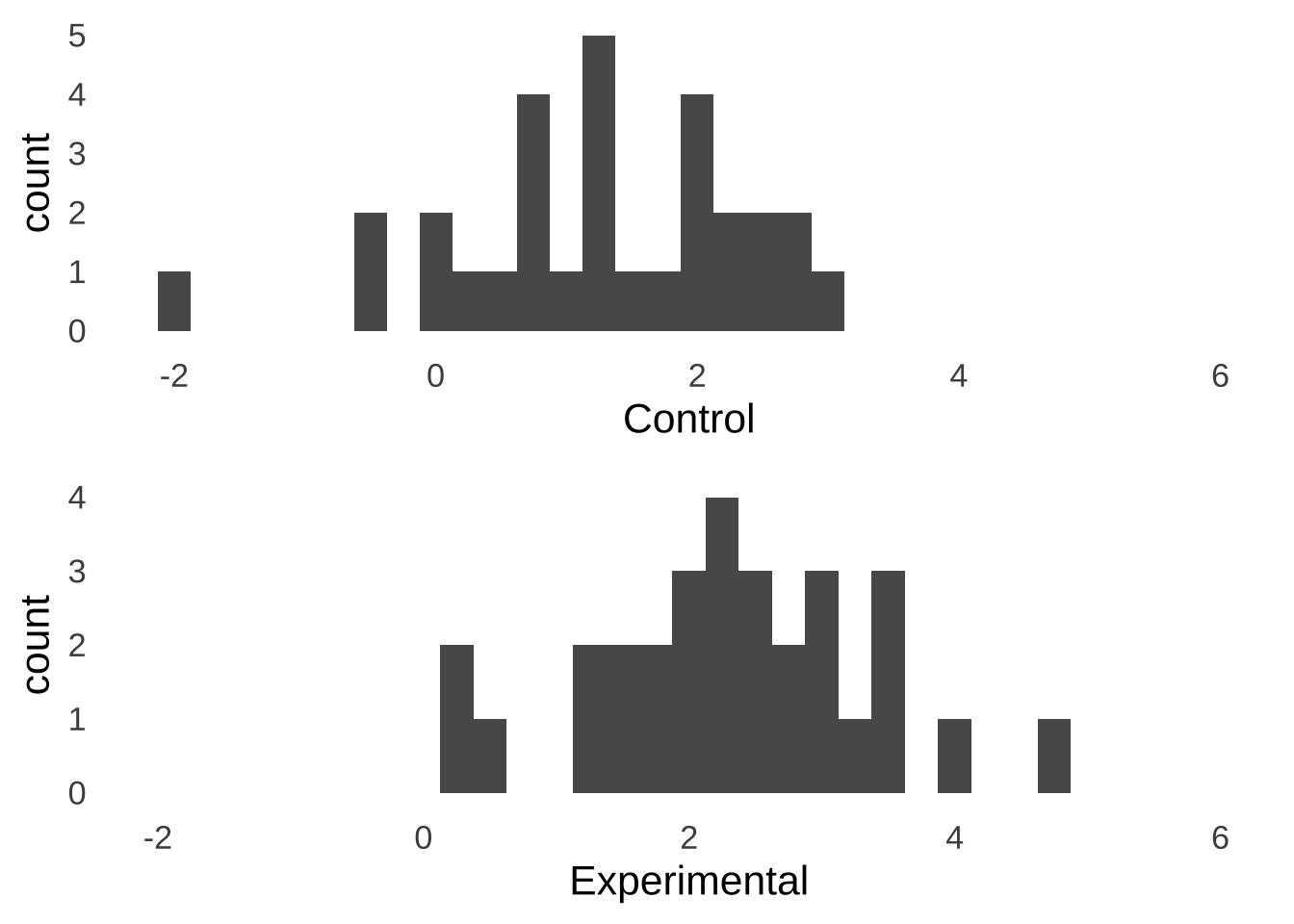
Figure 10.1: Hypothetical Experimental Data
Naturally, you want to know if there is a statistically significant difference between the mean of the control group and the mean of the experimental group. To test that difference, you decide to run an independent samples \(t\)-test on the data:
##
##  Two Sample t-test
##
## data:  Experimental and Control
## t = 3.6995, df = 58, p-value = 0.000482
## alternative hypothesis: true difference in means is not equal to 0
## 95 percent confidence interval:
##  0.4801216 1.6122688
## sample estimates:
## mean of x mean of y
##  2.296369  1.250174
The \(t\)-test says that there is a significant difference between the Experimental and Control groups: \(t(df=58)=3.7, p<0.01\). That’s a pretty cool result, and you may feel free to call it a day after observing it.
That one line of code – t.test(Experimental, Control, paired=FALSE, var.equal = TRUE) – will get you where you need to go. There may be other ways to analyze the observed data (for example: a nonparametric test or a Bayesian \(t\)-test), but that is a perfectly reasonable way to analyze the results of an experiment involving two separate groups of participants.
Using statistical software to calculate statistics like \(t\) and \(p\) is a little like riding a bicycle in that it takes some skill and it will get you to your destination fairly efficiently, but doing so successfully requires some assumptions. For the bicycle, it is assumed that there is air in the tires and the chain is on the gears and the seat is present: if those assumptions are not met, you still could get there, but the trip would be less than ideal. For the \(t\)-test – and for other classical parametric tests – the assumptions are about the source(s) of the data.
The \(t\)-test evaluates sample means using the \(t\)-distribution. It is based largely on the Central Limit Theorem, which tells that sample means are distributed as normals when \(n\) is sufficiently large…
\[\bar{x}\sim N\left(\mu, \frac{\sigma^2}{N} \right)\]
but it doesn’t tell us how large is sufficiently large. \(n=1,000,000\) would probably do it. The old rule of thumb is that \(n=30\) does it, but that is garbage.177
The only way to guarantee that the sample means – regardless of sample size – will be distributed normally is to sample from a normal distribution. We can prove that rather intuitively: imagine you had sample sizes of \(n-1\). The sample means for an \(n\) of 1 from a normal distribution would naturally be a normal distribution: it would be just like taking a normal distribution apart one piece at a time and rebuilding it (see Figure 10.2).
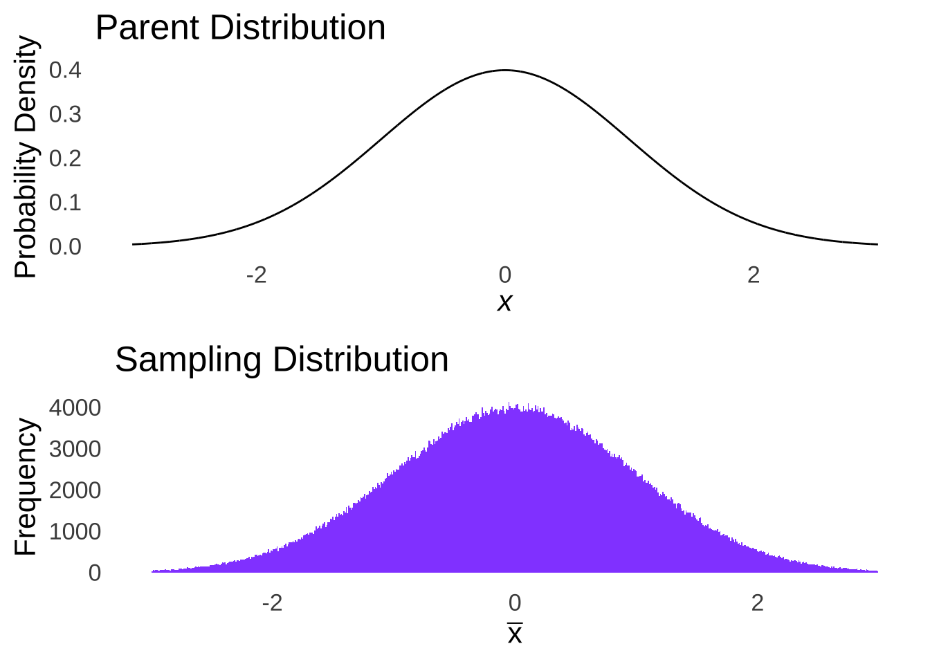
Figure 10.2: Normal Parent Distribution and Sampling Distribution with \(n=1\)
In the case of taking samples of \(n=1\) from a normal distribution, the distribution of sample means would be the same distribution we started with.178 This is the only distribution for which we can make such a claim. Hence: we assume that the data are sampled from a normal distribution.
The other feature that the use of the \(t\)-distribution to evaluate means depends on is the variance: as noted in Probability Distributions, the \(t\)-distribution models the distribution of sample means standardized by the sampling error. The standard deviation of a \(t\) distribution is the standard error, and, like the immortals in highlander…

Figure 10.3: This reference is \(almost\) too old even for me.
Thus, we assume that the data in the groups were drawn from populations with equal variances. This is known as either the homoscedasticity assumption or the homogeneity of variance assumption: take your pick (I prefer homoscedasticity because it’s more fun to say). Another way to view the importance of homoscedasticity is to consider what we would make of the results shown in Figure 10.1 if we knew that they came from the distributions shown in Figure 10.4:
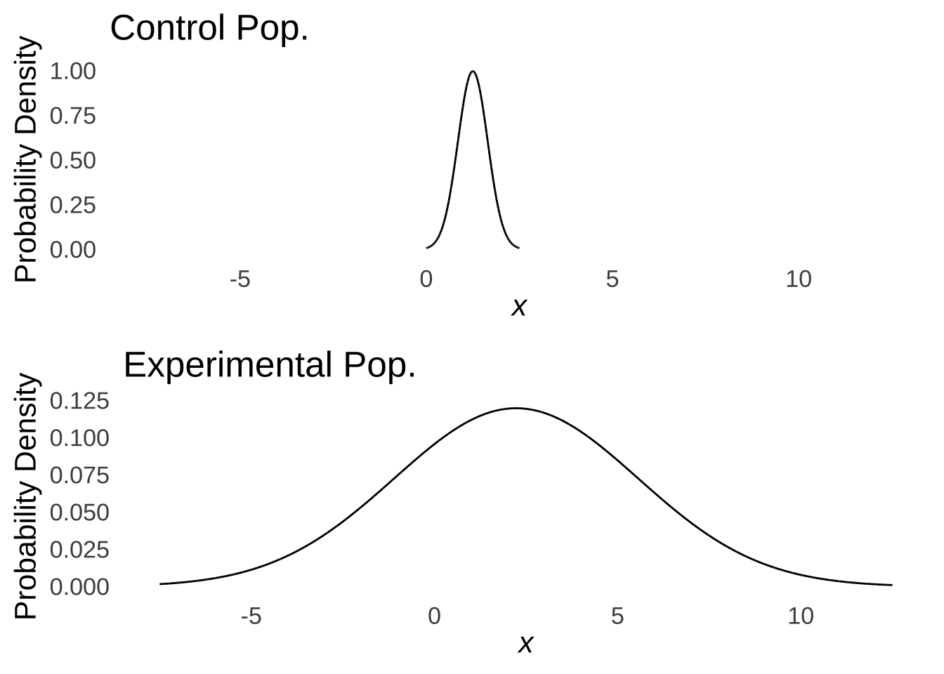
Figure 10.4: Populations with Means of 1.25 and 2.23, Respectively, and Very Different Variances
Were the populations to vary as in Figure 10.4, we might not be so sure about the difference between groups: it would appear that the range of possibilities in sampling from the Experimental population comfortably includes the entire Control population and that the difference is really of variances rather than means (which is not what we want to test with a \(t\)-test).
Maybe the simplest reason for assuming homoscedasticity is a research-methods reason: we want to assume that the only thing different about our populations is the experimental conditions. That is, all of our participants come in with their usual participant-to-participant difference with regard to the dependent measure (whatever it may be) and it is only the experimental manipulation that moves the means of the groups apart.
These assumptions undergird the successful use of the \(t\)-test. Like the bicycle – remember the bicycle analogy? – we can go ahead and use the \(t\)-test (or whatever other parametric test we are using) assuming that everything is structurally sound. If it gets us where we’re going: then violation of our assumptions probably didn’t hurt us too much. But, the responsible thing to do before riding your bicycle is to at least check your tire pressure, and the responsible thing to do before running classical parametric tests is to check your assumptions.
10.2 The General Assumptions
10.2.1 Scale Data
The classical parametric tests make inferences on parameters – means, variances, and the like – which are, by definition, numbers. To make inferences about numbers, we need data that are also numbers. Continuous data – interval- or ratio-level data – will work just fine. Ordinal data can also be used, but as discussed in Categorizing and Summarizing Information, it makes more logical sense to use nonparametric tests for ordinal data, as means and variances aren’t likely to be as meaningful for ordinal data as they are for continuous data.
10.2.2 Random Assignment
The classical parametric tests assume that in experimental studies with different conditions, that individual observations – be they observations of human participants, animal subjects, tissue samples, etc. – arise from random assignment to each of those experimental conditions. The key to random assignment is that individuals in a study should be on average the same with regard to the dependent variables.
For example, please imagine an educational psychology experiment involving undergraduate volunteers that tests the effect of two kinds of mathematics trainings – Program A and Program B – on performance on a problem set. If an experimenter were to find all of the math majors among the volunteers and to assign them all to the Program A group, we might not be surprised to see that Program A appears to have a more positive effect on problem set performance than Program B. That would not be random assignment. That would be cheating. If the volunteers were instead randomly assigned to groups, then, at least in theory, the levels of prior math instruction among participants would average out, and the condition means could be more meaningfully assessed.
10.2.3 Normality
The normality assumption is that the data are sampled from a normal distribution. This does not mean that the observed data themselves are normally distributed!
That makes testing the normality assumption theoretically tricky. While data that come from a normal distribution are not – and I can’t emphasize this enough – necessarily themselves normally distributed, we test the normality assumption by seeing whether the observed data could plausibly have come from a normal distribution. We do so with a classical hypothesis test, with the null hypothesis being that the data were sampled from a normal distribution, and the alternative hypothesis being that the data were not sampled from a normal distribution. So, it’s actually more accurate to say that we are testing the cumulative likelihood that the observed data or more extremely un-normal data were sampled from a normal distribution.
To summarize the above paragraph of nonsense: if the result of normality testing is not significant, then we are good with our normality assumption.
If the result is significant, then we have evidence that the data violate the normality assumption, in which case, we have options as to how to proceed.
Tests of normality are all based around what would be expected if the data were sampled from a normal distribution. The differences between different tests arise from the different sets of expectations they use. For example, on this page there are three tests of the normality assumption: the \(\chi^2\) goodness-of-fit test, the Kolmogorov-Smirnov test, and the Shapiro Wilk test. The \(\chi^2\) test is based on how many data points fall into different places based on what we would expect from a sample from a normal. The Kolmogorov-Smirnov test is based on how the observed cumulative distribution compares to a normal cumulative distribution. The Shapiro-Wilk test is based on correlations between observed data and data that would be expected from a normal distribution with the same dimensions. But the general idea of all these tests is the same: they compare the observed data to what would be expected if they were sampled from a normal: if those things are close, then we continue to assume our null hypothesis that the normality assumption is met, and if those things are wildly different, then we reject that null hypothesis.
10.2.3.1 Testing the Normality Assumption
10.2.3.1.1 The \(\chi^2\) Goodness-of-fit Test
The \(\chi^2\) goodness-of-fit test, as noted above, assesses where observed data points fall relative to each other. Let’s unpack that concept. One thing we know about the normal distribution is that 50% of the distribution is less than the mean and 50% of the distribution is greater than the mean:
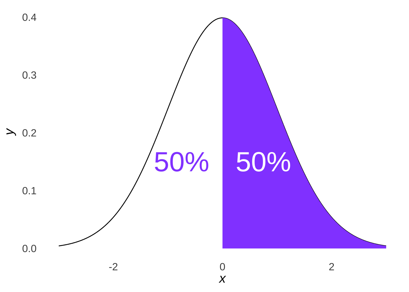
Figure 10.5: A Bisected Normal Distribution
Logically, it follows that if data are sampled from a normal distribution, roughly half should come from the area less than the mean and roughly half should come from the area greater than the mean. The distribution pictured in Figure 10.5, for example, is a standard normal distribution: were we to sample from that distribution, we would expect roughly half of our data to be less than 0 and roughly half to be greater than 0.
Likewise, if we divided a normal distribution into four parts, as in Figure 10.6…
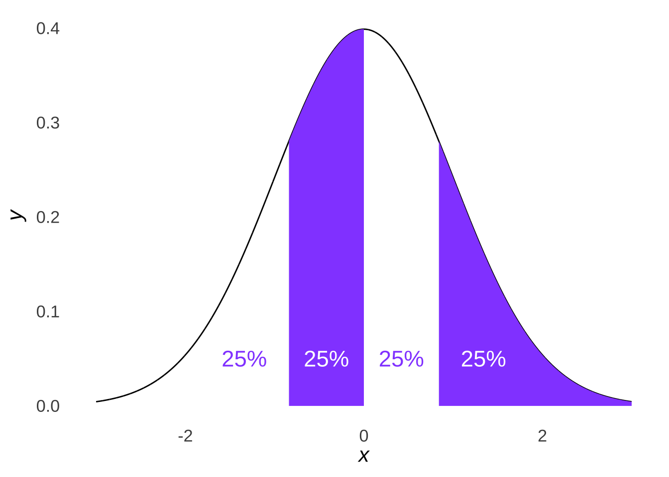
Figure 10.6: A Tetrasected Normal Distribution
… we would expect roughly a quarter of our data set to fall into each quartile of a normal distribution:
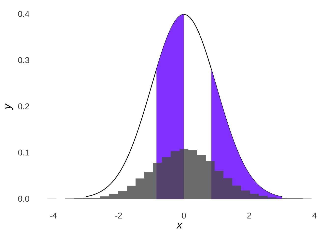
Figure 10.7: Four Parts of a Standard Normal Distribution Overlaid with a Histogram of 10,000 Samples from a Standard Normal Distribution
Whereas if we drew samples from a non-normal distribution like the \(\chi^2\) distribution (just because it’s known to be skewed – the fact that it’s in the \(chi^2\) test section is just a nice coincidence), we would see that the samples do not line up with the normal distribution with the same mean and standard deviation:
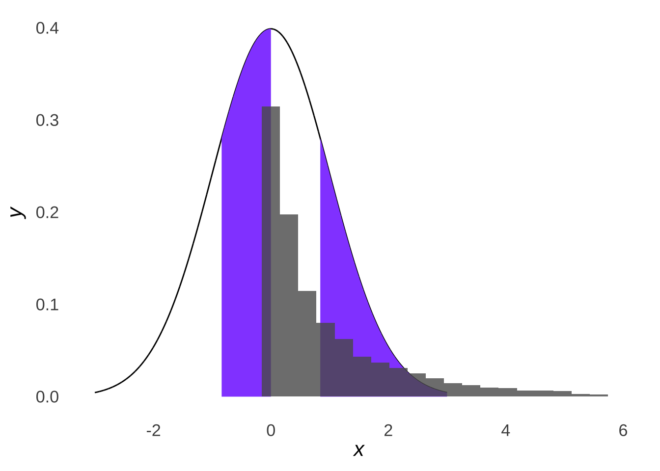
Figure 10.8: Four Parts of a Normal Distribution with \(\mu=1\) and \(\sigma=2\) Overlaid with a Histogram of 10,000 Samples from a \(\chi^2\) Distribution with \(df=1\) (\(\mu=1,~\sigma=2\))
Thus, the \(\chi^2\) goodness-of-fit test assesses the difference between how many values of a dataset we would expect in different ranges based on quantiles of a normal distribution and how many values of a dataset we observe in those ranges. We don’t know which normal distribution that the data came from179, but our best guess is that it is the normal with a mean equal to the mean of the observed data (\(\mu=\bar{x}_{observed}\)) and with a standard deviation equal to the standard deviation of the observed data (\(\sigma=s_{observed}\)).
To perform the \(\chi^2\) goodness-of-fit test, we divide the assumed distribution – in this case, the normal distribution with a mean equal to the observed sample mean and a standard deviation equal to the observed sample standard deviation – into \(k\) equal parts, divided by quantiles (if \(k=4\), then the quantiles are quartiles, if \(k=10\), then the quantiles are deciles, etc.). As an example, consider the following made-up observed data:
| 1.6 | 3.7 | 5.1 | 6.7 |
| 2.1 | 4.5 | 5.6 | 7.3 |
| 2.2 | 4.6 | 5.7 | 7.8 |
| 2.3 | 4.8 | 6.3 | 8.1 |
| 2.8 | 4.9 | 6.6 | 9.0 |
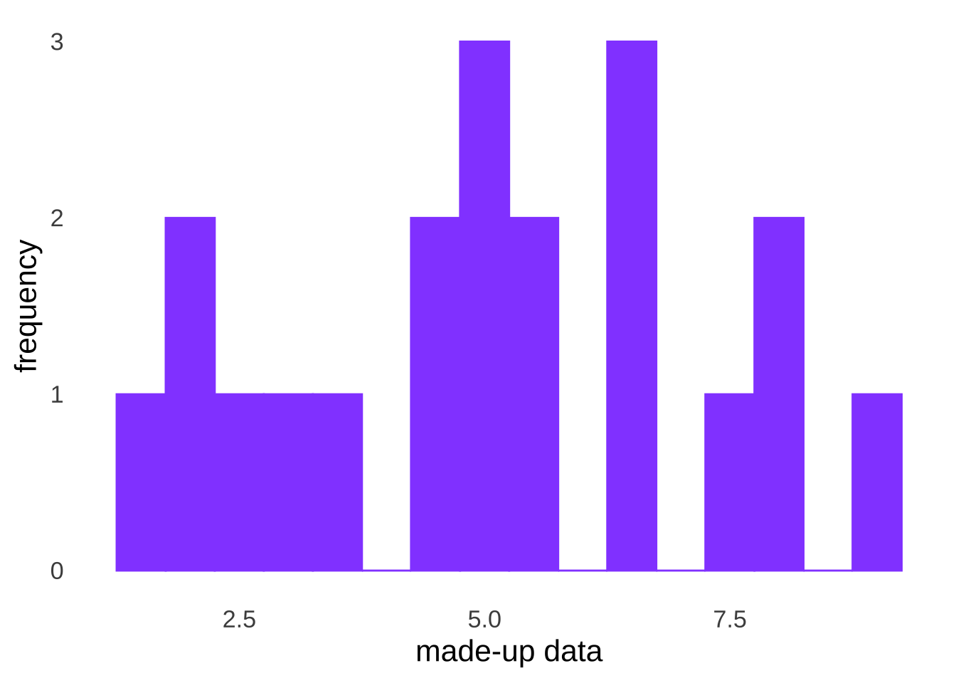
The mean of the made-up observed data is 5.08 and the standard deviation of the made-up observed data is 2.16. If we decide that \(k=4\) for our \(\chi^2\) test, then we want to find the quartiles for a normal distribution with a mean of 5.08 and a standard deviation of 2.16.
## [1] 3.623102 5.080000 6.536898For \(k\) groups – which we usually call cells – we expect about \(n/k\) observed values in each cell. The \(\chi^2\) test is based on the difference between the observed frequency \(f_e\) in each cell and the expected frequency \(f_o\) in each cell. The statistic known as the observed chi-squared statistic (\(\chi^2_{obs}\)) is the sum of the ratio of the square of the difference between \(f_o\) and \(f_e\) to \(f_o\) – the squared deviation from the expectation normalized by the size of the expectation:
\[\chi^2_{obs}=\sum\frac{(f_o-f_e)^2}{f_e}\]
The larger the difference between the observation and the expectation, the larger the \(\chi^2_{obs}\).
For the observed data, \(20/4=5\) value are expected in each quartile as defined by the normal distribution: 5 are expected to be less than 3.623102, 5 are expected to be between 3.623102 and 5.080000, 5 are expected to be between 5.080000 and 6.536898, and 5 are expected to be greater than 6.536898. The observed values are:
| \(-\infty \to 3.623\) | \(3.623 \to 5.080\) | \(5.080 \to 6.537\) | \(6.537 \to \infty\) |
|---|---|---|---|
| 5 | 5 | 4 | 6 |
The observed \(\chi^2\) value is:
\[\chi^2_{obs}=\sum\frac{(f_o-f_e)^2}{f_e}=\frac{(5-5)^2}{5}+\frac{(5-5)^2}{5}+\frac{(4-5)^2}{5}+\frac{(6-5)^2}{5}=0.4\]
The \(\chi^2\) test uses as its \(p\)-value the cumulative likelihood of \(\chi^2_{obs}\) given the \(df\) of the \(\chi^2\) distribution. The \(df\) is given by \(k-1\).180Thus, we find the cumulative likelihood of \(\chi^2_{obs}\) – the area under the \(\chi^2\) curve to the right of \(\chi^2_{obs}\) – given \(df=k-1\).
## [1] 0.9402425The \(p\)-value is 0.94 – nowhere close to any commonly-used threshold for \(\alpha\) (including 0.05, 0.01, and 0.001) – so we continue to assume the null hypothesis that the observed data were sampled from a normal distribution.
There is one point that hasn’t been addressed – why \(k=4\), or why any particular \(k\)? There are two things to keep in mind. The first is that a general rule for the \(\chi^2\) test is that it breaks down when \(f_e<5\): when the denominator of \(\frac{(f_o-f_e)^2}{f_e}\) is smaller than 5, the size of the observed \(\chi^2\) statistics can be overestimated. The second is that the larger the value of \(k\) – i.e., the more cells in the \(\chi^2\) test – the greater the power of the \(\chi^2\) test and the better the ability to accurately identify samples that were not drawn from normal distributions. Thus, the guidance for the size of \(k\) is to have few enough cells so that \(f_e \ge 5\), but as many more (or close to as many more) cells as possible.
10.2.3.1.2 The Kolmogorov-Smirnov Test
The Kolmogorov-Smirnov Test181 is a goodness-of-fit test that compares an observed cumulative distribution with a theoretical cumulative distribution. As illustrated in the page on probability distributions, the cumulative normal distribution is an s-shaped curve:
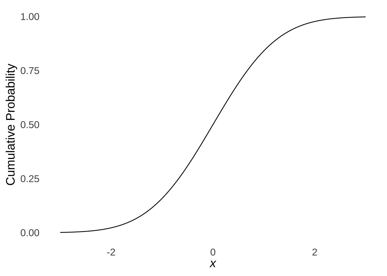
Figure 10.9: The Cumulative Standard Normal Distribution
To get the empirical cumulative distribution for a dataset, we order the data from smallest to largest. The first value in the empirical distribution is the first value in the ordered dataset. The second value in the empirical cumulative distribution is the sum of the first two values in the ordered dataset, the third value in the empirical cumulative distribution is the sum of the first three values in the ordered dataset, etc, until the last value in the empirical cumulative distribution which is the sum of all values in the data. For example, here is the empirical cumulative curve of the sample data:
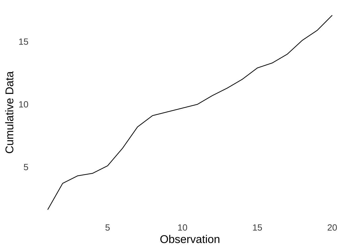
Figure 10.10: Empirical Cumulative Curve of the Made-up Data
The Kolmogorov-Smirnov test of normality is based on the differences between the observed cumulative distribution and the theoretical cumulative distribution with a mean equal to the mean of the sample data and a standard deviation equal to the standard deviation of the sample data. More specifically, the test statistic is the maximum difference between the observed and theoretical cumulative distributions (wich a couple of rules to determine what to do about ties in the data); this statistic is called \(D\). How the \(p\)-value is determine is a bit too unnecessarily complicated, especially because the Kolmogorov-Smirnov test is applied pretty easily using software. As shown below, the ks.test() command in the base R package takes as entry data the observed data, the cumulative probability distribution that the data are to be compared to – for a test of normality, this is the cumulative normal known to R as “pnorm” – and the sufficient statistics for the cumulative probability distribution – again, for normality: the mean and the standard deviation, which are given by the mean and standard deviation of the observed data.
data<-c(1.6, 2.1, 2.2, 2.3, 2.8, 3.7, 4.5, 4.6, 4.8, 4.9, 5.1, 5.6, 5.7, 6.3, 6.6, 6.7, 7.3, 7.8, 8.1, 9.0)

ks.test(data, "pnorm", mean(data), sd(data))
##
## Exact one-sample Kolmogorov-Smirnov test
##
## data: data
## D = 0.10489, p-value = 0.9639
## alternative hypothesis: two-sidedAs with the \(\chi^2\) test, the \(p\)-value is large by any standard, and thus we continue to assume that the data were sampled from a normal distribution.
10.2.3.1.3 The Shapiro-Wilk Test
The Shapiro-Wilk test is based on correlations between the observed data and datapoints that would be expected from a normal distribution with a mean equal to the mean of the observed data and a standard deviation equal to the standard deviation of the observed data.182
Unlike the \(\chi^2\) and Kolmogorov-Sminov test, the Shapiro-Wilk test is specifically made for testing normality, and its implementation in R is the simplest of the three tests:
data<-c(1.6, 2.1, 2.2, 2.3, 2.8, 3.7, 4.5, 4.6, 4.8, 4.9, 5.1, 5.6, 5.7, 6.3, 6.6, 6.7, 7.3, 7.8, 8.1,
9.0)

shapiro.test(data)
##
## Shapiro-Wilk normality test
##
## data: data
## W = 0.96466, p-value = 0.640610.2.3.2 Testing Normality for Multiple Groups
A lot of the parametric tests that we use – correlation, regression, independent-samples \(t\)-tests, ANOVA, and more – test the associations or differences between multiple samples. However, for each classical parametric analysis, there is only one normality assumption: that all the data are sampled from a normal. For example: were we interested in an analysis of an experiment with three conditions, we would not run three normality tests. We would only run one.
Of course, if there are multiple groups, each with different means, the data will not look like they came from a single normal, as in the pooled data from samples from three different normal distributions depicted in Figure 10.11.
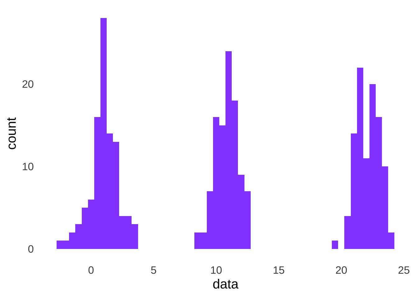
Figure 10.11: Distribution of the Combination of Three Groups of Data, Each Sampled From a Different Normal Distribution
And we run the Shapiro-Wilk test on all the observed data, we reject the null hypothesis: the pooled data violate the normality assumption.
##
##  Shapiro-Wilk normality test
##
## data:  data
## W = 0.86785, p-value = 2.349e-15
The solution to this problem is to not assess the observed data, but rather to assess the residuals of the data. The residuals of any group of data are the differences between each value in the group minus the group mean (\(x-\bar{x}\)). Because the mean is the balance point of the data, the mean of the residuals of any data set will be equal to 0. When we calculate and then put together the residuals of the 3 groups depicted in Figure 10.11:
then we have a single group of data with a mean of 0, as depicted in Figure 10.12.
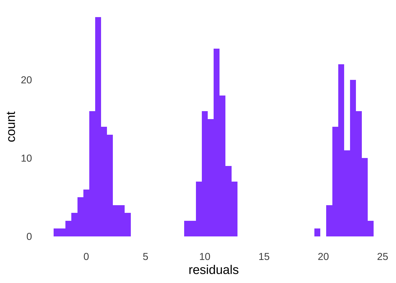
Figure 10.12: Distribution of the Combined Residuals of Three Groups of Data, Each Sampled From a Different Normal Distribution
And running a goodness-of-fit test on the residuals, we find that the assumption of normality holds:
##
##  Shapiro-Wilk normality test
##
## data:  residuals
## W = 0.99431, p-value = 0.3251
It should be noted that we need to run normality tests on the residuals – rather than the observed data – when we are assessing the normality assumption before running parametric tests with multiple groups. We don’t have to calculate residuals when testing the normality assumption for a single data set but we could without changing the results. Subtracting the mean of a dataset from each value in that set only changes the mean of the dataset from whatever the mean is to zero (unless the mean of the dataset is already exactly zero, in which rare case it would remain the same). Changing the mean of a normal distribution does not change the shape of that normal distribution, it just moves it up or down the \(x\)-axis. When we change the mean of an observed dataset, we also change the mean of the comparison normal distribution for the purposes of normality, and the both the shape of the data and the shape of the comparison distribution remain the same. So, for a single set of data, since the residuals will have the same shape as the observed data, we can run tests of normality on either the residuals or the observed data and get the same result – it’s only for situations with multiple groups of data that it becomes an issue.
10.2.3.3 Comparing Goodness-of-fit Tests
Of the three goodness-of-fit tests, the \(\chi^2\) test is the most intuitive (admittedly a relative achievement). It is also extremely flexible: it can be used not just to assess goodness-of-fit to a normal distribution, but to any distribution of data, so long as expected values can be produced to compare with observed values. It is also the least powerful of the three tests when it comes to testing normality – regardless of how many cells are used – and as such is the most likely to miss samples that violate the assumption that the data are drawn from a normal distribution.
The Kolmogorov-Smirnov test, like the \(\chi^2\) test, is not limited to use with the normal distribution. It can be used for any distribution for which a cumulative theoretical distribution can be produced. It is also more powerful than the \(\chi^2\) test and therefore less likely to miss violations of normality. Put those facts together and the Kolmogorov-Smirnov test is the most generally useful goodness-of-fit test of the three.
The Shapiro-Wilk test is the most powerful of the three and the easiest to implement in software. The only drawback to the Shapiro-Wilk test is that it is specifically and exclusively designed to test normality: it is useless if you want to assess the fit of data to any other distribution. Still, if you want to test normality, and you have a computer to do it with, the Shapiro-Wilk test is the way to go.
10.2.3.4 Visualizing Normality Tests: the Quantile-Quantile (Q-Q) Plot
A quantile-quantile or Q-Q plot is a visual representation of the comparison between an observed dataset and the theoretical probability distribution (such as the normal) to which it is being assessed. In a Q-Q plot such as the one in Figure 10.13 that depicts the goodness-of-fit between the made-up example data and a normal distribution, quantiles (such as \(1/n\), as used in Figure 10.13, to depict each observed data point) of the observed data are plotted against the counterpart quantile of the comparison distribution. If the two distributions are identical, then the points on the Q-Q plot precisely follow the 45\(^\circ\) diagonal line indicating that the quantiles are perfectly aligned. Departures from the diagonal can provide information about poor fits to the distribution being studied (the normal, for one, but a Q-Q plot can be drawn for any distribution one wants to model): systematic departures – like all of the points being above or below the diagonal for a certain region, or curvature in the plot – can give information about how the observed data depart from the selected model and/or clues to what probability distributions might better model the observed data.
In the case of the sample data, though, the observed data are well-modeled by a normal distribution: there is good goodness-of-fit, and we continue to assume that the data are sampled from a normal distribution.
data<-c(1.6, 2.1, 2.2, 2.3, 2.8, 3.7, 4.5, 4.6, 4.8, 4.9, 5.1, 5.6, 5.7, 6.3, 6.6, 6.7, 7.3, 7.8, 8.1,
9.0)
qqnorm(data)
qqline(data, col="#9452ff")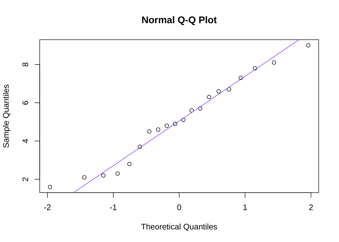
Figure 10.13: Quantile-Quantile Plot of the Goodness-of-Fit Between the Made-up Data and a Normal Distribution
10.2.4 Homoscedasticity (a.k.a. Homogeneity of Variance)
In parametric tests involving more than one group (including the independent-groups \(t\)-test and ANOVA) assume that the data in those groups are all sampled from distributions with equal variance. This assumption implies in an experimental context that even though group means might be different in different conditions, everybody was roughly equivalent before the experiment started; in a comparison of two different populations, we assume that each population has equal variance (but not necessarily equal means).
10.2.4.1 Testing Homoscedasticity
10.2.4.1.1 Hartley’s \(F_{max}\) Test
Hartley’s \(F_{max}\) test assesses homoscedasticity using the ratio of observed sample variances, specifically: the ratio of the largest variance to the smallest variance.183If all observed sample variances are precisely equal, then all evidence would point to homoscedasticity, and the ratio of the largest variance to the smallest variance (or technically, of any pair of variances if they are all identical) is 1. Of course, it is extraordinarily unlikely that any two sample variances would be exactly identical – even if two samples came from the same distribution, they would probably have at least slightly different variances.
Hartley’s test examines the departure from a variance ratio of 1, with greater allowances for departures given for combinations of small sample size and higher number of variances. The test statistic is the observed \(F_{max}\), and it is compared to a critical \(F_{max}\) value given the \(df\) of the smallest group and the number of groups.184
For example, assume the following data from two groups are observed:
| Placebo | Drug |
|---|---|
| 3.5 | 3.4 |
| 3.9 | 3.6 |
| 4.0 | 4.3 |
| 4.0 | 4.5 |
| 4.7 | 4.8 |
| 4.9 | 4.8 |
| 4.9 | 4.9 |
| 4.9 | 5.0 |
| 5.1 | 5.1 |
| 5.1 | 5.2 |
| 5.3 | 5.2 |
| 5.4 | 5.4 |
| 5.4 | 5.5 |
| 5.6 | 5.5 |
| 5.6 | 5.6 |
| 5.7 | 5.7 |
| 6.0 | 5.7 |
| 6.0 | 5.7 |
| 6.6 | 6.3 |
| 7.8 | 8.1 |
The variance of the placebo group is 0.98, and the \(df\) is \(n-1=19\). The variance of the drug group is 0.96, and the \(df\) is also \(n-1=19\). The observed \(F_{max}\) statistic – the ratio of the larger variance to the smaller – is:
\[obs~F_{max}=\frac{0.98}{0.96}=1.02\]
We can consult an \(F_{max}\) table to find that the critical value of \(F_{max}\) for \(df=19\) and \(k=2\) groups being compared is 2.53. Equivalently, we can use the qmaxFratio() command from the SuppDists packages, entering our desired \(\alpha\) level, the \(df\), the number of groups \(k\), and indicating lower.tail=FALSE, which is marginally faster than consulting a table:
## [1] 2.526451The critical \(F_{max}\) is the largest possible value of \(F_{max}\) given the \(df\) of the smallest group, the desired \(\alpha\) level, and the number of groups \(k\). Since the critical \(F_{max}\) for \(df=19\), \(k=2\), and \(\alpha=0.05\) is 2.526451, and the observed \(F_{max}\) value – 1.02 – is less than the critical \(F_{max}\), then we continue to assume that the data were sampled from populations with equal variance.
The only potential drawback to Hartley’s \(F_{max}\) test is that it assumes normality. If we’re testing normality anyway, that’s not a big deal! But, if you want to test homoscedasticity without being tied to assuming normality as well, might I recommend…
10.2.4.2 The Brown-Forsythe Test and Levene’s Test
The Brown-Forsythe test of homogeneity is an analysis of the variance of the absolute deviations – the absolute value of the difference between each value and its group mean \(|x-\bar{x}|\) – of different groups. Literally! The Brown-Forsythe test is an ANOVA of the absolute deviations. We reject the null hypothesis – and therefore the assumption of homoscedasticity – if the differences between all of the group variances are significantly greater than the variances observed within each group.
Levene’s test is based on the same concept as the Brown-Forsythe test, but can use deviations either from the median or the mean of each group. The leveneTest() command from the car (Companion to Applied Regression) package, by default, uses the median. The bf.test() command from the onewaytests package is related to the Brown-Forsythe test of homoscedasticity, but returns misleading results when group medians differ. Therefore, use the leveneTest() command to test homoscedasticity!
The Levene test command leveneTest() accepts data arranged in a long data frame format. In a wide data frame, the data from different groups are arranged in different columns; in a long data frame, group membership for each data point in a column is indicated by a grouping variable in a different column. For example, the following pair of tables show the same data in wide format (left) and in long format (right):
| Group A | Group B | Group | Data |
|---|---|---|---|
| 1 | 4 | Group A | 1 |
| 2 | 5 | Group A | 2 |
| 3 | 6 | Group A | 3 |
| Group B | 4 | ||
| Group B | 5 | ||
| Group B | 6 |
To put the two-group example data into long format, and to the run the Brown-Forsythe test on the variances of those data, takes just a few lines of R code:
library(car)
Placebo<-c(3.5, 3.9, 4.0, 4.0, 4.7, 4.9, 4.9, 4.9, 5.1, 5.1, 5.3, 5.4, 5.4, 5.6, 5.6, 5.7, 6.0, 6.0, 6.6, 7.8)

Drug<-c(3.4, 3.6, 4.3, 4.5, 4.8, 4.8, 4.9, 5.0, 5.1, 5.2, 5.2, 5.4, 5.5, 5.5, 5.6, 5.7, 5.7, 5.7, 6.3, 8.1)

lt.example<-data.frame(Group=c(rep("Placebo", 20), rep("Drug", 20)), Data=c(Placebo, Drug))
leveneTest(Data~Group, data=lt.example)
## Levene's Test for Homogeneity of Variance (center = median)
## Df F value Pr(>F)
## group 1 0.0891 0.767
## 3810.3 What to do When Assumptions are violated
If we test the assumptions regarding our data prior to running classical parametric tests, and we find that the assumptions have been violated, there are a few options for how to proceed.
First, we can collect more data. Although the Central Limit Theorem does not support prescribing any specific sample size to alleviate our assumption woes, it does imply that sample means based on larger sample size are more likely to be normally distributed, so the normality assumption becomes less important.
Second, we may transform the data, a practice encountered in the page on Correlation and Regression. Transformations can be theory-based, as in variables like sound amplitude and seismic intensity where the nature of the variables indicate that transformations of data are better analyzed using parametric tests than the raw data themselves. In other cases, transformations of data can reveal things about the variables. More theory-agnostic methods are available, such as the Cox-Box set of transformations185, but transformations without theoretical underpinnings are harder to justify.
Third, and I think this is the best option, is to use a nonparametric test. We’ll talk about lots of those.
Finally, as noted above: parametric tests tend to be robust against violations of the assumptions. A type-II error tends to me more likely than a type-I error, so if the result is significant, there’s probably no harm done. The danger is more in not observing an effect that you would have observed were the data more in line with the classical assumptions.
I had learned that the \(n=30\) guideline came from the work of Gosset and Fisher – and printed that in a book – but after re-researching there’s not a lot of hard evidence that either Gosset or Fisher explicitly told anybody to design experiments with a minimum \(n\) of 30. The only source I can find that cited a possible source for the origin of the claim linked to either Gosset or (noted dick) Fisher is the Stats with Cats blog.↩︎
The resulting distribution from repeatedly sampling single values from a normal distribution is the same as the original distribution mathematically speaking. I don’t know if it would be the same philosophically speaking or if that would be some kind of Ship of Theseus deal.↩︎
One of the central tenets of classical statistics is that we never know precisely what distribution observed data come from.↩︎
Why \(k-1\)? The \(\chi^2\) test measures membership of observations in \(k\) cells. Given the overall \(n\) of values, if we know the frequency of values in \(k-1\) cells, then we know how many values belong to the \(kth\) cell.↩︎
Just in case you encounter the term Lilliefors test, the Lilliefors test isn’t quite the same as the Kolmogorov-Smirnov test, but close enough that the tests are often considered interchangeable.↩︎
Saying that the Shapiro-Wilk test is based on “correlations” is understating the complexity of the test. A full description of the mechanics of the test – one that is much better than I could provide – is here.↩︎
The ratios of two variances are distributed as \(F\)-distributions. The maximum possible ratio between any two sample variances is the ratio of the largest variance to the smallest variance (the ratio of any other pair of variances would necessarily be smaller). Hence, the term \(F_{max}\).↩︎
The \(df\) in this case is the \(n\) per sample minus 1. When assessing a sample variance, the \(df\) is based on how the sample mean (which is a part of the sample variance calculation \(\sigma^2=\frac{\sum(x-\bar{x})^2}{n-1}\)) is calculated. When determining cell membership as for the \(\chi^2\) test, if we know how many of \(n\) values are in \(k-1\) cells, we then know how many values are in the \(kth\) cell; when determining group means, if we know the sample mean and \(n-1\) of the numbers in the group, then we know the value of the \(nth\) number, so \(df=n-1\). The underlying idea is the same, but the equations are different based on the needs of the test.↩︎
If you think it’s funny that Cox and Box collaborated on papers, you’re not alone: George Cox and David Box thought the same thing and that’s why they decided to work together.↩︎