Chapter 9 Markov Chain Monte Carlo Methods
9.1 Let’s Make a Deal
In the September 9, 1990 issue of Parade Magazine, the following question appeared in Marilyn vos Savant’s “Ask Marilyn” column:
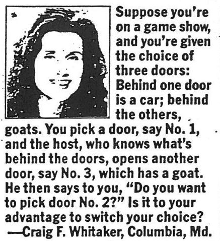
This is the most famous statement of what came to be known as The Monty Hall Problem due to the similarity of its setup to the game show Let’s Make a Deal, hosted in the 60’s, 70’s, 80’s, and 90’s by Monty Hall. This article lays out the history of the problem and the predictably awful reason why vos Savant in particular drew so voluminous and vitriolic a response for her correct answer (hint: it rhymes with “mecause she’s a woman”).
The Monty Hall Problem is set up nicely for solving with Bayes’s Theorem. In this case, we are interested in comparing:
- the posterior probability that the prize is behind the door originally picked by the contestant and
- the posterior probability that the prize is behind the door that the contestant can switch to.
For simplicity of explanation, let’s say that the contestant originally chooses Door #1, and the host shows them that the prize is not behind Door #2 (the answer is the same regardless of what specific doors we choose to calculate the probabilities for). Thus, we are going to compare the probability that the prize is behind Door 1 given that the host has shown that the prize is not behind Door 2 – we’ll call that \(p(Door_1|Show_2)\) – with the probability that the prize is behind Door 3 given that the host has shown Door 2 – \(p(Door_3|Show_2)\).
The prior probability that the prize is behind door #1 is \(p(Door_1)=1/3\) and the prior probability that the prize is behind Door #3 \(p(Door_3)\) is also \(1/3\) – without any additional information, each door is equally likely to be the winner.
Since the contestant has chosen Door #1, the host can only show either Door #2 or Door #3. If the prize is in fact behind Door #1, then each of the host’s choices are equally likely, so \(p(Show_2|Door_1)=1/2\). However, if the prize is behind Door #3, then the host can only show Door #2, so \(p(Show_2|Door_3)=1\). Thus, the likelihood associated with keeping a choice is half as great as the likelihood associated with switching.
The base rate is going to be the same for both doors, so it’s not 100% necessary to calculate, but here it is anyway: \(p(Show_2)=p(Door_1)p(Show_2|Door_1)+p(Door_3)p(Show_2|Door_3)=1/2\).
Thus, the probability of Door #1 having the prize given that Door #2 is shown – and thus the probability of winning by staying with the original choice of Door #1 – is:
\[p(Door_1|Show_2)=\frac{(1/3)(1/2)}{1/2}=\frac{1}{3}\]
and the probability of the prize being behind Door #3 and thus the probability of winning by switching is:
\[p(Door_3|Show_2)=\frac{(1/3)(1)}{1/2}=\frac{2}{3}\].
What does this have to do with Monte Carlo simulations? Well, the prominent mathematician Paul Erdös famously refused to believe that switching was the correct strategy until he saw a Monte Carlo simulation of it. so that’s what we’ll do.
9.2 Let’s Make a Simulation, or, the Monte Carlo Problem
9.2.1 Single Game Code
Let’s start by simulating a single game.
First, let’s randomly put the prize behind a door. To simulate three equally likely options, we’ll draw a random number between 0 and 1: if the random number is between 0 and \(1/3\), that will represent the prize being behind Door 1, if the random number is between \(1/3\) and \(2/3\), that will represent the prize being behind Door 2, and if the random number is between \(2/3\) and 1, that will represent the prize being behind Door 3.
The default sufficient statistics in the base R distribution commands with the root unif() define a continuous uniform distribution that ranges from 0 to 1. Using the command runif(1) will take one sample from that uniform distribution: it’s a random number between 0 and 1. We can use the ifelse command to record a value of 1, 2, or 3 for the simulated prize location:
## Putting the prize behind a random door

set.seed(123) ## Setting a specific seed makes the computer take the same random draw each time the program is run - very helpful if you're making a web page and need the answers to be consistent.

x1<-runif(1)     ## Select a random number between 0 and 1
Prize<-ifelse(x1<=1/3, 1, ## If the number is between 0 and 1/3, the prize is behind Door 1
              ifelse(x1<=2/3, 2, ## Otherwise, if the number is less than 2/3, the prize is behind Door 2
                     3))        ## Otherwise, the prize is behind Door 3

Prize
## [1] 1Next, we can simulate the contestant’s choice. Since the contestant is free to choose any of the three doors and their choice is not informed by anything but their own internal life, we can use the same algorithm that we used to place the prize:
## Simulating contestant's choice

x2<-runif(1)     ## Select a random number between 0 and 1
Choice<-ifelse(x2<=1/3, 1, ## If the number is between 0 and 1/3, contestant chooses Door 1
              ifelse(x2<=2/3, 2, ## Otherwise, if the number is less than 2/3, contestant chooses Door 2
                     3))        ## Otherwise, contestant chooses Door 3

Choice
## [1] 3Now, here’s the key step: we simulate which door the host shows the contestant. It’s going to be a combination of rules and randomness:
- If the contestant has chosen the prize door, then the host shows either of the two other doors with \(p=1/2\) per door.
- We can draw another random number between 0 and 1: if it is less than \(1/2\) then one door is chosen, if it is greater than \(1/2\) then the other is chosen.
- If the contestant has not chosen the prize door, then the host must show the door that is neither the prize door nor the contestant’s choice:
x3<-runif(1)

if(Prize==1){
  if(Choice==1){
    ShowDoor<-ifelse(x3<=0.5, 2, 3)
  }
  else if(Choice==2){
    ShowDoor<-3
  }
  else{
    ShowDoor<-2
  }
} else if(Prize==2){
  if(Choice==1){
    ShowDoor<-3
  }
  else if(Choice==2){
    ShowDoor<-ifelse(x3<=0.5, 1, 3)
  }
  else{
    ShowDoor<-1
  }
} else if(Prize==3){
  if(Choice==1){
    ShowDoor<-2
  }
  else if(Choice==2){
    ShowDoor<-1
  }
  else{
  ShowDoor<-ifelse(x3<=0.5, 1, 2)
  }
}


ShowDoor
## [1] 2Given the variables Prize, Choice, and ShowDoor, we can make another variable StayWin1 to indicate if the contestant would win (StayWin = 1) or lose (StayWin = 0) by keeping their original choice:
## [1] 0And we can also create a variable SwitchWin2 to indicate if the contestin would win (SwitchWin = 1) or lose (SwitchWin = 1) by switching their choices:
if (Choice==1){
  if (ShowDoor==2){
    Switch<-3
  } else if (ShowDoor==3){
    Switch<-2
  }
} else if (Choice==2){
  if (ShowDoor==1){
    Switch<-3
  } else if (ShowDoor==3){
    Switch<-1
  }
} else if (Choice==3){
  if (ShowDoor==1){
    Switch<-2
  } else if (ShowDoor==2){
    Switch<-1
  }
}

SwitchWin<-ifelse(Prize==Switch, 1, 0)
SwitchWin
## [1] 1Thus, to recap, in this specific random game: the prize was behind Door #1, the contestant chose Door #3, and the host showed Door #2: the contestant would win by switching and lose by staying. But, that’s just one specific game: in games where stochasm is involved, good strategies often lose and bad strategies often win.^[“My shit doesn’t work in the play-offs. My job is to get us to the play-ffs. What happens after that is fucking luck”
– Billy Beane, characterizing the difference between stochastic strategy in large vs. small sample sizes. from Lewis, M. (2003) Moneyball. New York: W.W. Norton & Company, p. 275.]
9.2.2 Repeated Games
Now, let’s pull the whole simulation together and repeat it 1,000 times. If our simulation works (hopefully!) and Bayes’s Theorem works, too (hahaha it better!), then we should see about \(1/3\) of the 1,000 games won by staying and about \(2/3\) won by switching.
The following code takes all the lines of code for the single-repetition game and wraps it in a for loop with 1,000 iterations.
## Putting the prize behind a random door

StayWin<-rep(NA, 1000)   ## When making an array, R prefers if you define an empty array first.
SwitchWin<-rep(NA, 1000) ## We start with "NA's" - R's version of blanks - and we'll fill them in with our program

for (i in 1:1000){
x1<-runif(1)     ## Select a random number between 0 and 1
Prize<-ifelse(x1<=1/3, 1, ## If the number is between 0 and 1/3, the prize is behind Door 1
              ifelse(x1<=2/3, 2, ## Otherwise, if the number is less than 2/3, the prize is behind Door 2
                     3))        ## Otherwise, the prize is behind Door 3
## Simulating contestant's choice

x2<-runif(1)     ## Select a random number between 0 and 1
Choice<-ifelse(x2<=1/3, 1, ## If the number is between 0 and 1/3, contestant chooses Door 1
              ifelse(x2<=2/3, 2, ## Otherwise, if the number is less than 2/3, contestant chooses Door 2
                     3))        ## Otherwise, contestant chooses Door 3

x3<-runif(1)

if(Prize==1){
  if(Choice==1){
    ShowDoor<-ifelse(x3<=0.5, 2, 3)
  }
  else if(Choice==2){
    ShowDoor<-3
  }
  else{
    ShowDoor<-2
  }
} else if(Prize==2){
  if(Choice==1){
    ShowDoor<-3
  }
  else if(Choice==2){
    ShowDoor<-ifelse(x3<=0.5, 1, 3)
  }
  else{
    ShowDoor<-1
  }
} else if(Prize==3){
  if(Choice==1){
    ShowDoor<-2
  }
  else if(Choice==2){
    ShowDoor<-1
  }
  else{
  ShowDoor<-ifelse(x3<=0.5, 1, 2)
  }
}


StayWin[i]<-ifelse(Prize==Choice, 1, 0)

if (Choice==1){
  if (ShowDoor==2){
    Switch<-3
  } else if (ShowDoor==3){
    Switch<-2
  }
} else if (Choice==2){
  if (ShowDoor==1){
    Switch<-3
  } else if (ShowDoor==3){
    Switch<-1
  }
} else if (Choice==3){
  if (ShowDoor==1){
    Switch<-2
  } else if (ShowDoor==2){
    Switch<-1
  }
}

SwitchWin[i]<-ifelse(Prize==Switch, 1, 0)
}

MontyHallResults<-data.frame(c("Staying", "Switching"), c(sum(StayWin), sum(SwitchWin)))
colnames(MontyHallResults)<-c("Strategy", "Wins")
ggplot(MontyHallResults, aes(Strategy, Wins))+
  geom_bar(stat="identity")+
  theme_tufte(base_size=16, base_family="sans", ticks=FALSE)+
  labs(x="Strategy", y="Games Won")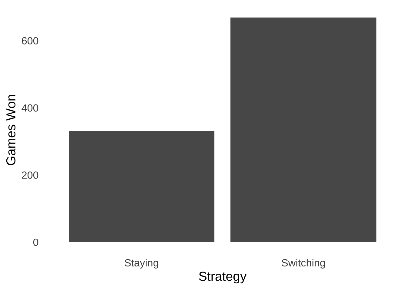
Figure 9.1: Frequency of Wins in 1,000 Monty Hall Games Following ‘Stay’ Strategies and ‘Switch’ Strategies
In our simulation, a player who stayed every time would have won \(331\) games for a winning percentage of \(0.331\); a player who switched every time would have won \(669\) games for a winning percentage of \(0.669\). So, Marilyn vos Savant and Thomas Bayes are both vindicated by our simulation.
Please note that we arrived at our simulation result without including anything in the code about Bayes’s Theorem or any other mathematical description of the problem. Instead, we arrived at estimates of the expected value of the distribution of wins by describing the logic of the game. That’s a valuable feature of MCMC methods: in situations where we might not have firm expectations for the posterior distribution of a complex process, we can arrive at estimates based on taking those processes step-by-step.
Another matter of interest (possibly only to me): the game described in the Monty Hall Problem was never really played on Let’s Make a Deal.
9.3 Random Walks
Random Walk models are an application of Monte Carlo Methods. Random Walks were introduced in the page on probability theory, but are worth revisiting. The random walk uses randomly-generated numbers to make models of stochastic3 processes. The model depicted in Figure 9.2 simulates the cash endowment of a gambler making repeated $10 bets on a 50-50 proposition: at each step, she can either win $10 or lose $10. In this series of gambles, the gambler starts with $100. Her cash endowment peaks at $170 after winning 8 out of her first 11 bets, she hits her minimum of $60 on four separate occasions (after losing her 65th, 67th, 125th, and 199th bets), and finishes with $70.
Figure 9.2: A Random Walk
The value of using a Random Walk model in this example is that it provides a tangible description of a set of behaviors that result from a stochastic process – this is a case where the behavior is of a hypothetical bankroll rather than of a human or an animal – that might not be as easily understood if described by statistics like the expected value and variance of a gamble.
In this example, the expected value of each gamble is 0 – one is just as likely to win $10 as to lose $10, the variance of each gamble is the probability-weighted square of the expectations: \((\frac{1}{2})(\$100)+(\frac{1}{2})(\$100)=\$100\) and the standard deviation is \(\sqrt{\$100}=\$10\). Thus, in the long run, the expectation of the gamble over \(N\) trials is \(0\times N\), the variance is \(\$100 \times N\), and the standard deviation is \(10 \times \sqrt{N}\).4 But, that doesn’t really give us an accurate description of the gambling experience, nor, by extension, of how people make decisions while gambling. If somebody went to a casino with $100, they might be less likely to want to know what would happen if I went to the casino an infinite amount of times and played an infinite amount of games? and more likely to know will I win?. With repeated Random Walk models – that is, running models like the one above 1,000 or 1,000,000 times or whatever we like – we can model the rate at which a gambler could run out of money, the rate at which they could hit a target amount of winnings at which they decide to walk away, or the rate of anything in-between.
The above is a relatively simple Random Walk, as it only involves one dimension, and we have ways of understanding long-term expected values of each step. Random Walks can also be two-dimensional, as in Figure 9.3, a demonstration of a two-dimensional random walk model from this paper on cellular biology:
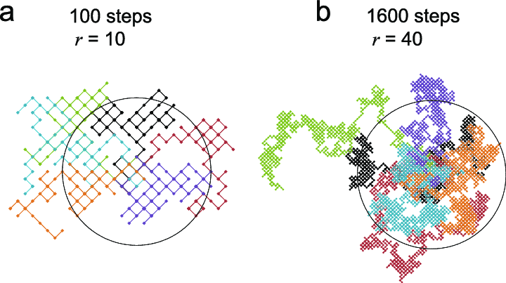
Figure 9.3: Diagram of Two-Dimensional Random Walk Model
9.4 Markov Chain Monte Carlo Methods
Random Walk models are, specifically, examples of Markov Chain Monte Carlo methods (MCMC). The key quality of Markov Chains is the condition of being memoryless. A Markov Chain is one in which the next step in a chain depends only on the current step. That is: each event is a step from the current state – a step in one dimension as in Figure 9.2, in two dimensions as in Figure 9.3 or more — that is independent of whatever steps that came before the current state.5
We also can use MCMC models as blunt-force tools for understanding stochastic processes where analytic methods come up short. Famously, mathematicians have been unable to use analytic methods to determine the probability of winning a game of Klondike Solitaire, (see Figure 9.4). Every time you start a new game, the result of the prior game has no bearing on the next one.
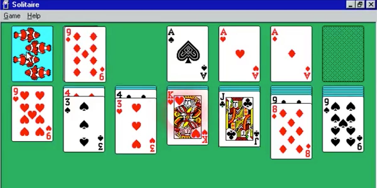
Figure 9.4: Solitaire is a Lonely Man’s Game.
By simulating games using Monte Carlo methods, computer scientists have found solutions to the Solitaire problem where mathematicians haven’t be able to.
Computer simulations of games more complex than Klondike – namely, athletic competitions – are often used in popular media to predict outcomes. For example: ESPN has used the Madden series of video games to simulate the outcome of Super Bowls. Letting computer-generated opponents play each other in a video game repeatedly is equivalent to a Monte Carlo simulation with lots of parameters, including simulated physical skills of the simulated competitors and the physics of the simulated environment. It’s also the basic plot generator of the 2006 film Rocky Balboa.
On the remote chance that you, dear reader, may be interested in statistical analysis regarding things other than game shows, or gamblers, or solitaire, or boxing matches, we turn now to the main point:
9.5 MCMC in Bayesian Analysis
MCMC methods are a popular way to estimate posterior distributions of parameters in Bayesian frameworks.^[MCMC methods are not very popular in frequentist statistics for several reasons, including:
Posterior distributions aren’t a thing in the frequentist framework, and
frequentist statistics are based around assumed, rather than estimated probability distributions.
There are classical methods that make use of repeated sampling, most prominently the calculation of bootstrapped confidence intervals, but these also rely on the assumption of probability distributions.] As described in Classical and Bayesian Inference, once the posterior distribution on a parameter (or set of parameters) is determined, then various inferential questions can be answered, such as: what is the highest density interval (HDI)? or what is the probability that the parameter is greater than/less than a variable of interest?
Here we will focus on the most flexible – although not always the most efficient – MCMC method for use in Bayesian inference: the Metropolis-Hastings (MH) algorithm. We will discuss how it works, how to get estimates of a posterior distrbution, why MH gives us samples from the posterior distribution, and applications to Psychological Science.
9.5.1 The Metropolis-Hastings Algorithm
Here’s a really super-basic explanation of how the MH algorithm works: you start with a random number for your model, then you pick another random number. If the new random number makes your model better, you keep it, if it doesn’t, then sometimes you keep it anyway but otherwise you stick with the old number. You repeat that process a bunch of times, keeping track of all the numbers that you kept, and the numbers you kept are the distribution.
The italicized step (sometimes you keep it anyway) is the key to generating a distribution. If the MH algorithm only picked the better number, then the procedure would converge on a single value rather than a distribution. What’s worse, that number might not be the best number, and the algorithm could get stuck for a long time until a better number is found. The sometimes is key to getting a distribution with both high-density probabilities and lower-density probabilities (a common feature of probability distributions).
9.5.1.1 Sampling from the Posterior Distribution
The random numbers that we plug into the MH algorithm are candidate values for parameters. We sample them at random from a prior distribution: in Bayesian terms, they are samples from \(p(H)\). The determination of whether the new candidate values make the model better or not is based on the likelihood of the observed data given the hypothesized values of the parameters: in Bayesian terms, it is the likelihood \(p(D|H)\). We decide which candidate value is better based on the ratio of the prior times the likelihood of the new candidate to the prior times the likelihood of the old candidate. If we call the current parameter value \(H_1\), the proposed new candidate parameter \(H_2\), and the ratio of the products of the priors and the likelihoods \(r\), then:
\[r=\frac{p(H_2)p(D|H_2)}{p(H_1)(p(D|H_2)}\] Since Bayes’s Theorem tells us that the posterior probability of \(H\) is \(\frac{p(H)p(D|H)}{p(D)}\), \(r\) is the ratio of the two posterior probabilities \(p(H_2|D)\) and \(p(H_1|D)\) – \(p(D)\) would be the same for both hypotheses, and so cancels out. If we sample all of the candidate values from the same prior distribution – as we will for our examples in this page – \(p(H)\) cancels out as well. For example, if each candidate value is sampled randomly from a uniform distribution, then the probability of choosing each value is the same. Thus, it is more common to present the ratio \(r\) as:
\[r=\frac{p(D|H_2)}{p(D|H_1)}\] Sampling parameter values from a prior distribution and evaluating them based on the product of the (often canceled) prior probability and the likelihood given the prior divided by the (always canceled) probability of the data ensures that the MH produces samples from the posterior distribution.
9.5.1.2 The Acceptance sub-Algorithm
The MH algorithm always accepts the proposed candidate parameter value if the likelihood of the data given the new parameter is greater than or equal to 1:
\[1.~Accept~H_2~if~r=\frac{p(D|H_2)}{p(D|H_1)}\ge1.\] Thus the posterior distribution will be loaded up with high-likelihood values of the parameter. The sometimes is also not nearly as random as my super-basic description has made it out to be.
As alluded to above, the MH algorithm sometimes accepts the proposed candidate parameter value if the likelihood of the data given the new parameter is less than 1. The new parameter will be accepted with a probability equal to the likelihood ratio: if \(r=0.8\), then the probability of accepting \(H_2\) is \(0.8\); if \(r=0.2\), then the probability of accepting \(H_2\) is \(0.2\). That is how the MH algorithm produces the target distribution based on the likelihood function: it doesn’t randomly accept parameters that don’t increase the likelihood of the data given the parameter, it accepts them at a rate equal to how close they get the model to peak likelihood.
The step of accepting parameters that don’t increase the likelihood at rates equal to the amount that they do change the likelihood is accomplished by generating a random value from a uniform distribution which is usually called \(u\). Similarly to how we simulated a choice between three doors by generating a random number from the uniform distribution and calling it (for example) “Door #1” if the random number were \(\le 1/3\), if \(r>u\), then we accept the proposed candidate value for the parameter:
\[2.~Accept~H_2~if~r=\frac{p(D|H_2)}{p(D|H_1)}>u,~else~accept~H_1\] If, for example, \(r=0.8\), because there is an 80% chance that the random number \(u<0.8\), there is an 80% chance that \(H_2\) will be accepted; if \(r=0.2\), then there is a 20% chance that \(H_2\) will be accepted because there is a 20% chance that a randomly-generated \(u\) will be less than \(0.2\).
Here, in words, is the full Metropolis-Hastings algorithm:
- Choose a starting parameter value. Call this the current value.
In theory, it doesn’t really matter which starting value you use – it can be a complete guess – but it helps if you have an educated guess because the algorithm will get to the target distribution faster if the starting parameter is closer to the middle of what the target distribution will be. For a parameter in the \([0, 1]\) range, \(0.5\) is a reasonable place to start.
- Generate a proposed parameter value from the prior distribution.
For example, given an uninformative prior, a sample from a uniform distribution will do nicely.
- Calculate the ratio \(r\) between the likelihood of the observed data given the proposed value to the and the likelihood of the observed data given the current value.
This part can be trickier than it appears. For the MH algorithm to generate the actual target distribution, it must use a good likelihood function (formally, this requirement is often stated the likelihood function must be proportional to the target distribution). In a case where the data are binomial, then the likelihood function is known (it’s the binomial likelihood function \(\frac{N!}{s!f!}\pi^s(1-\pi)^f\)). For more complex models, the likelihood function can be derived in much the same way the binomial likelihood function is derived. Other investigations can make assumptions about the likelihood function: if a normal distribution is expected to be the target distribution, for example, then the likelihood function is the density function for the normal (\(f(x|\mu, \sigma)=\frac{1}{\sigma \sqrt{2\pi}}e^{-\left( \frac{x-\mu}{\sigma} \right)^2}\)). But, once the likelihood function is decided upon, \(r\) is just a simple ratio of the likelihood given the proposed value to the likelihood given the current value.
- If \(r\ge 1\), accept the proposed parameter.
- If \(r>u(0, 1)\), accept the proposed parameter.
\(u(0,1)\) refers to a random number from a uniform distribution bounded by 0 and 1. When coding the MH algorithm, we can just call it \(u\).
- else, accept the current parameter.
The accepted parameter becomes the current parameter. Store the accepted parameter.
Repeat steps 1 – 5 as many times as you like.
How many iterations are used is somewhat a matter of preference, but there are a couple of considerations:
9.5.1.2.1 Model complexity
A model with a single parameter will generally require fewer samples for the MH algorithm to converge to the target distribution than models with two or more. Whereas 1,000 iterations might be enough to generate a smooth target distribution for a single parameter, 1,000,000 or more might be required in situations where two or more parameters have to be estimated simultaneously.
9.5.1.2.2 Burn-in Period
As noted above, the starting parameter value or values for the MH algorithm are guesses (educated or otherwise). The algorithm is dumb – it doesn’t know where it’s going, and if you happen to start it far away from the center of the target distribution, there may be some meaningless wandering at the beginning. This problem is more pronounced when there are multiple parameters. Thus, the first few iterations are often referred to as the burn-in period and are thrown out of estimates of the posterior distribution. As with the overall number of trials, there’s no a priori way of knowing how many iterations the burn-in period should last. For what it’s worth: I learned that the burn-in period should be about the first 3% of trials (presumably based on my stats teacher’s MCMC experience). Basically, you want to take out any skew caused by the first bunch of trials: if you drop them and the mean and sd of the distribution changes, they probably should be dropped, and if you drop more and the mean and sd stay the same, then you probably don’t need to drop the additional trials.
9.5.1.2.3 Auto-correlation
Getting stuck in place is a concern for MH models when there are multiple parameters involved: when the combination of multiple parameters need to increase the posterior likelihood to have a high chance of being accepted, there can be long periods of continuing to accept the current parameters. The concern there is that some parameters could inappropriately be overrepresented by virtue of the search algorithm getting stuck. That concern is easily alleviated by taking every \(nth\) iteration (say, every 100th value of the parameters), but doing so might require taking increased overall iterations and more computing time.6
The following code performs the MH algorithm on data from a binomial experiment where \(s=16\) and \(f=4\) (note: these are the same data from the Classical and Bayesian Inference page). Figure ?? illustrates the selection process of the algorithm for 1,000 iterations. For this example, we know that the target distribution is a \(\beta\) distribution with a mean of \(\frac{s+1}{s+f+2}\approx 0.77\) and a standard deviation of \(\sqrt{\frac{\hat{\pi}(1-\hat{\pi})}{s+f+3}}\approx 0.088\). Please note that the accepted values of the parameter (which is called theta in the code) accumulate near the center of the target distribution but occasionally less likely values are accepted.
set.seed(77)
s<-16
N<-20
theta<-c(0.5, rep(NA, 999))
for (i in 2:1000){ #Number of MCMC Samples
  theta2<-runif(1) #Sample theta from a uniform distribution
  ltheta2<-dbinom(s, N, theta2) ## p(D|H) for new theta
  ltheta1<-dbinom(s, N, theta[i-1]) #p(D|H) for old theta
  r<-ltheta2/ltheta1 #calculate likelihood ratio

  u<-runif(1) #Sample u from a uniform distribution
  theta[i]<-ifelse(r>=1, theta2, #replace theta according to MH algorithm
                   ifelse(r>u, theta2, theta[i-1]))
}
x<-1:1000
theta<-data.frame(theta, ltheta2, x)
Figure 9.5: Results of 1,000 Markov Chain Monte Carlo Samples Selected Using the Metropolis-Hastings Algorithm
The mean of the posterior distribution generated by the MH algorithm is 0.78 and the standard deviation is 0.086 – very close to the analytic solution from the posterior \(\beta\) distribution that has a mean of 0.77 and a standard deviation of 0.088.
Now that we have some test cases to indicate that the algorithm works and how it works, let’s review a couple of useful applications for estimating posterior distributions on parameters: multinomial models and regression.
9.6 Multinomial Models
Multinomial Models are tools for describing the relationships between latent processes and observable outcomes. For example, multinomial models are often used in genetics research: genotypes are generally latent (they were way more latent before modern microscopy), while phenotypes are observable. If Gregor Mendel had computers and knew of Markov Chain Monte Carlo methods (both of which were invented after he died), he might have used the Metropolis-Hastings algorithm (also posthumous for our monk friend) to model the distribution of dominant and recessive genes in pea plants.
Psychology, of course, encompasses the study of many unobservable latent processes. We can’t directly measure how much a person stores in their memory nor how likely they are to be able to access what they have stores, but we can measure what stimuli they can recall or recognize. We can’t directly measure how people perceive different features of a stimulus but we can measure what features they can identify.
Multinomial models in psychology presuppose that multiple processes can occur in the mind with different probabilities and map out the combination or combinations of processes that need to occur to produce an observable outcome (like a behavior). For example, a multinomial memory model might posit that to remember somebody’s name, one would have to A. have stored that person’s name in their memory and B. be able to retrieve it from memory. In that model, if it is assumed that a stimulus is either stored or is not, then there is a probability of storage in memory and the probability of non-storage is 1 minus that probability.7 Then, there is a probability of retrieval and a probability of non-retrieval (\(1-p(retrieval)\)). The goal of multinomial modeling is to recover those probabilities based on observable behaviors. Those probabilities can be used to describe latent processes under different conditions. To continue with the memory example: if our research question is how do memory processes change as a function of time?, we may compare the posterior distribution of \(p(storage)\) at time \(t\) with the posterior distribution of \(p(storage)\) at time \(t+1\), the posterior distribution of \(p(retrieval)\) at time \(t\) with the posterior distribution of \(p(retrieval)\) at time \(t\), etc.
Multinomial models are naturally described using probability trees. Figure 9.6 is an example of a relatively basic generic multinomial model.
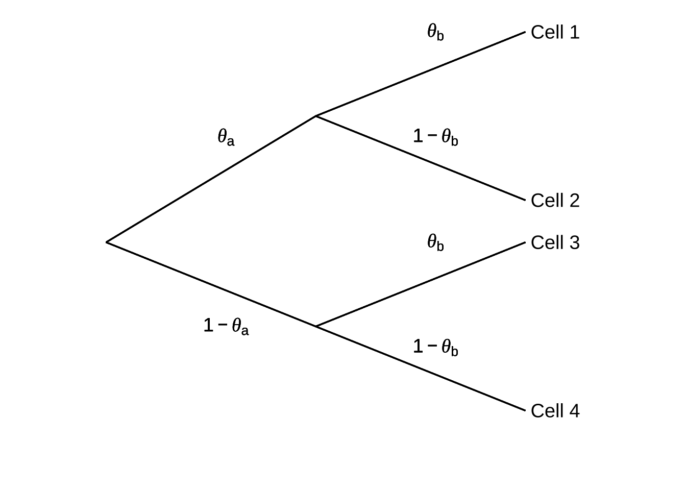
Figure 9.6: Generic Tree Representation of a Multinomial Model (adapted from Batchelder & Reifer, 1999)
In this model, for the behaviors noted in Cell 18 to occur, two events need to happen: one with probability \(\theta_a\) and another with probability \(\theta_b\). Thus, behavior 1 (recorded in Cell 1) happens with probability \(\theta_a \theta_b\). Behavior 2 happens with probability \(\theta_a(1-\theta_b)\), behavior 3 happens with probability \((1-\theta_a)\theta_b\), and behavior 4 happens with probability \((1-\theta_a)(1-\theta_b)\).
The blessing and the curse of multinomial models is that they are flexible enough to handle a wide range of theories of latent factors. If there are, say, four possible processes that could occur in the mind at a given stage of the process, one can construct a multinomial model with four branches coming off of the same node. If different paths can lead to the same behavior (for example, remembering a fact can help you on a multiple choice test but guessing can get you there – less reliably – too), one can construct a multinomial model where multiple paths end in the same outcome. A multinomial model can take on all kinds of forms based on the theory of the latent processes that give rise to observable phenomena like behaviors and physiological changes: that’s the blessing. The curse is that we have to come up with likelihood functions that fit the models, which can be a chore.
For the model in Figure 9.6, the likelihood function is structurally similar to the binomial likelihood function: we take the probabilities involved in getting to each end of the paths in the model and multiply them by the number of ways we can go down those paths. That is, the likelihood function is the product of a combinatorial term and a kernel probability term.
Let’s say we have an experiment with \(N\) trials, where \(n_1,~n_2,~n_3,\) and \(n_4\) are the number of observations of behaviors 1, 2, 3, and 4, respectively. The combinatorial term – \(N\) things combined \(n_1\), \(n_2\), and \(n_3\) at a time (with \(n_4\) technically being leftover) is:
\[\frac{N!}{n_1!n_2!n_3!n_4!}\] The kernel probability is given by the product of each probability – \(\theta_a\), \(\theta_b\), \(1-\theta_a\), and \(1-\theta_b\) – raised to the power of the cells in which they play a part in getting to:
\[\theta_a^{n_1+n_2}\theta_b^{n_1+n_3}(1-\theta_a)^{n_3+n_4}(1-\theta_b)^{n_2+n_4}\]
Thus, our entire likelihood function for the model, where cells are represented by \(\n_i\) is:
\[{\cal L}(\theta_a, \theta_b)=p(D|H)=\frac{N!}{n_1!n_2!n_3!n_4}\theta_a^{n_1+n_2}\theta_b^{n_1+n_3}(1-\theta_a)^{n_3+n_4}(1-\theta_b)^{n_2+n_4}\] We can make a user-defined function in R to calculate \({\cal L}(\theta_a, \theta_b)\):
likely<-function(n1, n2, n3, n4, theta.a, theta.b){
  L<-(factorial(n1+n2+n3+n4)/(factorial(n1)*factorial(n2)*factorial(n3)*factorial(n4)))*
    (theta.a^(n1+n2))*
    (theta.b^(n1+n3))*
    ((1-theta.a)^(n3+n4))*
    ((1-theta.b)^(n2+n4))
  return(L)
}
Now, we will run an experiment.
Actually, we don’t have time for that. Let’s suppose that we ran an experiment with \(N=100\) and that these are the observed data for the experiment:
| Observation | \(n\) |
|---|---|
| Cell 1 | 28 |
| Cell 2 | 12 |
| Cell 3 | 42 |
| Cell 4 | 18 |
And let’s estimate posterior distributions for \(\theta_a\) and \(\theta_b\) using the MH algorithm. Note that in this algorithm, we have two starting/current parameter values and two proposed parameter values, corresponding to \(\theta_a\) and \(\theta_b\). At each iteration, we plug values for both parameters into the likelihood function and either accept both proposals or keep both current values. This tends to slow things down a bit, but is more flexible than algorithms that change one parameter at a time.9 Given that we have two parameters to estimate, for this analysis we will use 1,000,000 iterations.
iterations<-1000000

theta.a<-c(0.5, rep(NA, iterations-1))
theta.b<-c(0.5, rep(NA, iterations-1))

n1=28
n2=12
n3=42
n4=18

for (i in 2:iterations){
  theta.a2<-runif(1)
  theta.b2<-runif(1)
  r<-likely(n1, n2, n3, n4, theta.a2, theta.b2)/likely(n1, n2, n3, n4, theta.a[i-1], theta.b[i-1])
  u<-runif(1)
  if (r>=1){
  theta.a[i]<-theta.a2
  theta.b[i]<-theta.b2
  } else if (r>u){
  theta.a[i]<-theta.a2
  theta.b[i]<-theta.b2
  } else {
    theta.a[i]<-theta.a[i-1]
    theta.b[i]<-theta.b[i-1]
  }
  }
Assuming a burn-in period of 3,000 iterations, here are the estimated posterior distributions of \(\theta_a\) and \(\theta_b\) given the observed data:
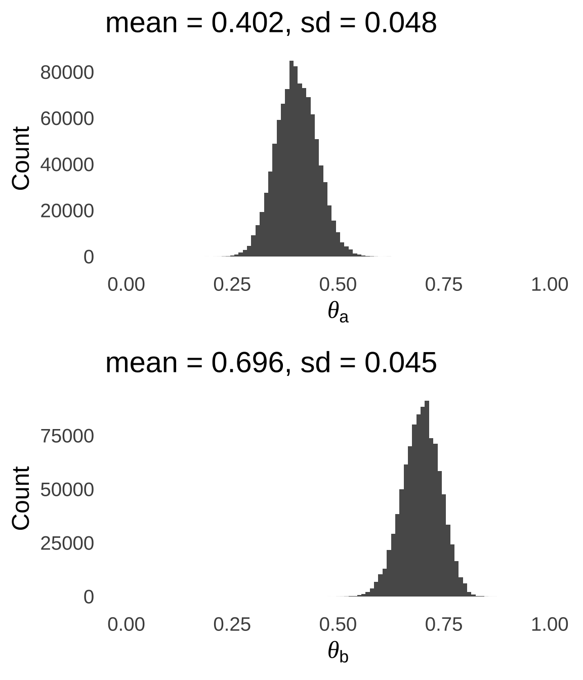
Figure 9.7: Posterior Distributions of \(\theta_a\) and \(\theta_b\) Given the Observed Data
As a check, let’s plug the mean values of \(\theta_a\) and \(\theta_b\) back into our multinomial model to see if they result in predicted data similar to our observed data:
| Observation | \(n_{obs}\) | \(p(\phi_i)\) | \(n_{pred}\) |
|---|---|---|---|
| Cell 1 | 28 | \(\theta_a \theta_b\) | 27.997 |
| Cell 2 | 12 | \(\theta_a(1-\theta_b)\) | 12.201 |
| Cell 3 | 42 | \((1-\theta_a)\theta_b\) | 41.651 |
| Cell 4 | 18 | \((1-\theta_a)(1-\theta_b)\) | 18.151 |

9.7 Bayesian Regression Models
Regression models are the last application of MCMC we will cover here. In the context of regression, the likelihood function is related to the fit of the model to the data. For example, in classical linear regression, the likelihood function is the product of the normal probability density of the prediction errors: the least-squares regression line is the model with parameters that maximize that likelihood function.10
Bayesian regression confers a couple of advantages over its Classical counterpart. Because Bayesian models don’t assume normality, there is less concern about using it with variables sampled from different distributions, and since the results are not based on the normal assumption, Bayesian regression outputs can include more informative interval estimates on model statistics like the slope and the intercept (for example: non-symmetric interval estimates where appropriate). Another advantage is that Bayesian interval estimates are often more narrow than classical estimates in cases where MCMC methods give more precise measurements than classical methods, which, again, assume that model statistics are sampled from normal distributions. Finally (there are more I can think of but I will stop here out of a sense of mercy), Bayesian point and interval estimates have more intuitive interpretations than classical estimates.
Bayesian regression using MCMC is complex in theory, but easily handled with software. Using the BAS package, for example, we can use many of the same commands that we use for classical regression to obtain Bayesian models.
As an example, let’s use the data represented in Figure 9.8.
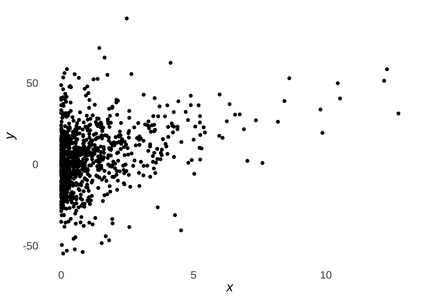
Figure 9.8: Sample Scatterplot
First, let’s run a classical simple linear regression with the base R lm() commands. Instead of the full model summary() command, we will limit our output by using just the coef() command to get the model statistics and the confint() command to get interval estimates for the model statistics.
## (Intercept)           x
## 0.2589419 3.8024346## 2.5 % 97.5 %
## (Intercept) -1.042028 1.559912
## x 3.127986 4.476884Next, we will use the Bayesian counterpart bas.lm() from the BAS package, with 500,000 MCMC iterations11:
##               2.5%    97.5%     beta
## Intercept 3.260162 5.387505 4.363655
## x         3.106006 4.435586 3.795684
## attr(,"Probability")
## [1] 0.95
## attr(,"class")
## [1] "confint.bas"
The results are very similar! The Bayesian interval estimate for the coefficient of \(x\) (that is, the slope) is slightly narrower than the classical confidence interval, but for the Bayesian interval, you’re allowed to say “there’s a 95% chance that the parameter is between 3.1 and 4.4.” The intercept is slightly different, too, but that has little to do with the differences between Bayesian and classical models and much more to do with the fact that the BAS package uses an approach called centering which forces the intercept to be the mean of the \(y\) variable – it’s a choice that is also available in classical models and one that isn’t going to mean a whole lot to us right now.
And that’s basically it. There are lots of different options one can apply regarding different prior probabilities and Bayesian Model Averaging (which, as the name implies, gives averaged results that are weighted by the posterior probabilities of different models, but is only relevant for multiple regression), but for basic applications, modern software makes regression a really easy entry point to applying Bayesian principles to your data analysis.
At this point, I feel compelled to admit that I’m not very good at naming variables.↩︎
Like, I’m really bad at naming variables↩︎
As a reminder: stochastic means probabilistic in the sense that is the opposite of deterministic – that is: the outcomes in a stochastic process are not determined by a series of causes leading to certain effects but by a series of causes leading to possible effects.↩︎
Variances add linearly, standard deviations do not.↩︎
Recall from Probability Theory that the Random Walk is also known as the Drukard’s Walk: none of the steps that have gotten somebody who is blackout drunk to where they are predict the next step they will take.↩︎
Your experiences may vary with regard to how much additional computing time may be incurred by increasing the number of MCMC iterations. If a lot of MCMC investigations are being run, the time can add up. In the case of a single analysis of a dataset, it’s probably more like an excuse to get up from your computer and have a coffee break while the program is running. ↩︎
A more complicated memory model might posit that there is also a chance of partial storage, as in the phenomenon when you can remember the first letter or sound of somebody’s name.↩︎
“Cell” is used in this case in the same sense as “cells” in a spreadsheet where data are recorded.↩︎
There is a specific subtype of the Metropolis-Hastings algorithm known as the Gibbs Sampler that does hold one parameter constant while changing the other at each iteration. The upside is that the Gibbs Sampler can be more computationally efficient, the downside is that the Gibbs Sampler requires assumptions about the conditional distributions of each parameter given the other and thus is less broadly useful than the generic MH algorithm. It’s fairly popular among Bayesian analysts and it’s not unlikely that you will encounter it, but the MH algorithm can always get you – eventually – where you need to go.↩︎
Not to get too into what I meant to be a brief illustration, but it might be confusing that we want to maximize a function based on the errors when the goal of regression modeling is to minimize the errors generally. The link there is that the normal probability density is highest for values near the mean of the distribution; and if the mean of the errors is 0, then minimizing the errors maximizes the closeness of the errors to the mean – and thus the peak – of the normal density.↩︎
Without getting too far into the mechanics of the
BASpackage, it uses a subset of MH-generated samples to estimate statistics and intervals.↩︎