Chapter 4 Probability Theory

4.1 Probability, Statistics, and Scientific Inquiry

Let’s do a thought experiment. Please imagine that I am a charming rapscallion who has drawn international curiosity for my boastful claims that I can read minds and that you are a skeptical scientist interested in investigating my abilities or lack thereof. Suppose I offer to prove my telepathy by asking you to draw from a well-shuffled deck of 52 standard playing cards: you are to draw a card, to look at it, and not to show me what it is.

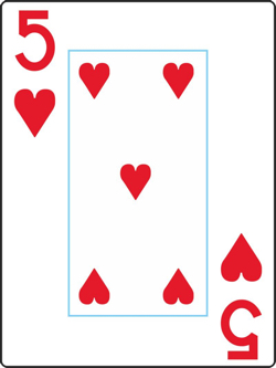
Figure 4.1: your card

In this hypothetical scenario, your card is the five of hearts.

Now suppose I make one of the following claims:

You have drawn either a red card or a black card.
You have drawn a red card.
You have drawn a heart.
You have drawn the five of hearts.

All of those claims are equally correct. The five of hearts – which again, is your card – is either red or black, is red, is a heart, and is the five of hearts. But as we proceed from claim 1 down to claim 4, the statements probably seem more convincing to you. We may be convinced by, say, claim 4 but not claim 1, is that each claim differs not in whether it is correct or not but by the boldness of each claim. The bolder of these claims offer more details; with more details, the probability of being correct by guessing goes down. Let’s evaluate the probability that I could correctly make each claim if I didn’t have the power to read minds:

4.1.0.0.1 You have drawn either a red card or a black card.

All playing cards are either red (hearts or diamonds) or black (clubs or spades). So this claim has to be true. The probability of getting this right is 100%. This one is dumb. Let’s move on.

4.1.0.0.2 You have drawn a red card.

Half of the playing cards in a deck are red (hearts and diamonds). If I were guessing at random, I would have a 50% chance of getting this one right. That’s not terribly impressive but it’s slightly better than the first claim.

4.1.0.0.3 You have drawn a heart.

One-fourth of the playing cards in a deck are hearts, so the probability of getting this right by guessing randomly is 25%. That might make you say something like, “hey, good guess,” but it’s probably not enough to make you think that I have mutant powers. Next!

4.1.0.0.4 You have drawn the five of hearts.

There’s only one five of hearts in the deck. Given that there are 52 cards in a standard deck, the probability of randomly guessing any individual card and matching the one that was drawn is therefore $1/52$: a little less than 2%. Since there are 51 cards in the deck that are not the five of hearts, the probability that I am wrong is $51/52$: a little more than 98%. In other words, it is 51 times more likely that I would guess incorrectly by naming a single, specific card than that I would guess correctly. That’s fairly impressive – at this point one might be wondering if it’s a magic trick or I am otherwise cheating or possibly that I might have an extra sense, but either way one might start ruling out the possibility that I am guessing purely at random.

Now let’s say that I have made claim 4 – that you have drawn the five of hearts – and that I am correct. You, still the scientist in this scenario, skeptical though you may be, decide to share your assessment of my unusual (and, to be clear, fictional) talent with the world. You write up the results of this card-selecting-and-guessing experiment and have it published in an esteemed scientific journal. In that article, you say that I have the ability to read minds, or, at least, the part of minds that store information about recently-drawn playing cards. But, you include the eminently reasonable caveat that you could be wrong about that; it may be a false alarm. In fact, you know that if I were a fraud and I were merely guessing, that given the assumptions that the deck was standard and every card was equally likely to be drawn, the likelihood of me being right was $1/52$.

On the other hand, there is no way to be 100% certain that I have the ability to read minds. Maybe you’re not satisfied with the terms of our little experiment and you think they would lead to false alarms too often for your liking. So, maybe we do the same thing with two decks of cards. The probability of me naming your card from one deck and repeating with another deck is much smaller than performing the feat with just one deck (we’ll learn about this later on, but it’s $\frac{1}{52}\times\frac{1}{52}=\frac{1}{2,704}$, or about 0.04%). As we add more decks to the experiment, the probability of correctly guessing one card from each one approaches zero – but never equals zero.

There is one other implication to this thought experiment that I would like to point out. Often it is not practical, feasible, or possible to replicate our scientific studies. Let’s say we only have one shot at our mind-reading experiment: we only have one deck of cards, and for some reason, we can only use it once (so, no replacing the card, reshuffling, and trying again). If we would not consider identifying a single card correctly as sufficient evidence of telepathy – and, to be sure, a 1/52 chance is by no means out of the realm of possibility – there is a way to incorporate our skepticism into the evaluation of the probability of true telepathy with the observation of card identification. We’ll talk about this in the section on Bayesian Inference.

As you (back to real you, no longer the hypothetical you of our fantastical scenario) may have inferred, this thought experiment is meant to serve as an extended metaphor for probability, statistics, and scientific inquiry. We are nearly never certain about the results of our studies: there is always some probability involved, be it a probability that our hypotheses are correct and supported by the data, a probability that our hypotheses are correct but not supported by the data, a probability that our hypotheses are incorrect and not supported by the data, and/or a probability that our hypotheses are incorrect but supported by the data anyway.

Statistics are our way to assess those probabilities. Not every investigation is based on knowable and calculable probabilities like our example of guessing cards – in fact, almost all of them are not. There are many, many statistical procedures precisely because most scientific studies are not associated with relatively simple probability structures like there is a one-out-of-fifty-two chance that the response is just a correct guess.

So: first, we are going to learn the rules of probability and we are going to use a lot of examples like decks of cards and marbles and jars and coin flips (SO MANY COIN FLIPS) to help us. As we proceed on to learning more statistical procedures, the fundamental goal will be the same: understanding the probability that the thing that we are observing is real.

4.2 The Three Kolmogorov (1933) Axioms

4.2.1 1. Non-negativity

The probability of an event⁵⁸ must be a non-negative real number.

\[p(A)\in \Re;~p(A)\ge0\]

In other words, a probability value can’t be negative. I might say that there is a $-99%$ chance that I am going to go to a voluntary staff meeting at 6 am, but that is just hyperbole and is not physically possible (the probability is actually 0). Imaginary numbers are impossible for probabilities, too, so if at any point in this semester you find yourself answering a probability problem with $p=\sqrt{-0.87}$, please check your work.

4.2.2 2. Normalization

The sum of all possible mutually exclusive events in a sample space⁵⁹ is 1.

So, as long as multiple events can’t happen at the same time, the sum of the probability of all of the events is one.

\[\sum{\Omega}=1\]

4.2.3 3. Finite Additivity

The probability of the co-occurrence of two mutually exclusive events⁶⁰ is equal to the sum of the probabilities of each event:

\[if~p(A~and~B)=0,~p(A+B)=p(A)+p(B)\]

and since the principle extends to more than two mutually exclusive events, we could also extend the above equation to $p(A\cup B\cup C)$, and $p(A\cup B\cup C\cup D)$, etc.

This axiom allows us to add the probabilities of events based on the fact that the sum of mutually exclusive events is the sum of the probabilities: for example, a coin can’t land heads and tails on the same flip, so the probability of heads or tails is $0.5+0.5=1$.

4.3 Methods of Assigning Probability

There are several methods of assigning a probability value to an event. All methods agree on the probability assigned to heads vs. tails in a flip of a fair coin, but they may disagree on the probabilities of other events. We can largely categorize these methods as objective – methods that depend solely on mathematical calculations – or subjective – methods that take into account what people believe about events.

4.3.1 Objective Methods

4.3.1.1 Equal Assignment

In the equal assignment of probability, each elementary event in a sample space is considered equally probable. This is the method used for games of chance, including coin flips, dice rolls, and card games. So, when we say that the probability of heads is 0.5, or the probability of rolling a 7 with a pair of dice is $1/6$, or the probability of drawing an ace from a shuffled deck is $1/13$, we are assigning equal probability to each possible elementary outcome.

4.3.1.2 Relative Frequency

Relative frequency theory bases the probability of something happening on the number of times it’s happened in the past divided by the number of times it could have happened. For example, imagine that you had never seen or heard of a fair coin before, let alone thought to flip one, and did not know that there were two equally probable outcomes to a coin flip. Without being able to assign equal probability theory, you could come to understand the probability of heads and tails by flipping the coin (presumably after being shown how to do so) many times. After enough flips, the relative numbers of heads and tails would converge to an equal number of occurrences.

4.3.2 Subjective Probability

A subjective probability is a statement of the degree of belief in the probability of events. Any time we put a number to the chances of an event in our personal lives – the probability that we remembered to lock the door when we left home, the probability that we will finish a paper by Friday, the probability that we will feel less-than-perfect after a night of revelry – we are making a statement of subjective probability.

Subjective probability is not based on wild guesses – when we make subjective probability statements about our own lives they tend to be based on some degree of self-awareness – and in science, subjective probability judgments tend to incorporate data and some objective measures of probability as well. Meteorologists are a classic example: a statement like there is a 40% chance of rain is based on a subjective interpretation of weather models that incorporate terabytes of data on things like climate, atmospheric conditions, prior weather events, etc. A statistician who uses subjective methods may use their judgment in choosing probabilistic models and starting points, but ultimately makes their decisions based on objective data.

4.4 Intersections and Unions

The distinction between the conjunctions and and or has important implications in interpersonal communication: if somebody asks you want for dessert, whether you reply with I want cake OR pie or I want cake AND pie may have serious consequences for the amount of food you get. The same is true for determining the probability of multiple events.

4.4.1 Intersections

In probability theory (as well as in formal logic and other related fields) the concept of co-occurring events, e.g., event $A$ and event $B$ happening, is known as the intersection⁶¹ of those events and is represented by the symbol cap $\cap$. The probability of event $A$ and event $B$ happening is thus equivalently expressed as the intersection probability of $A$ and $B$, as $p(A)\cap~p(B)$, and as $p(A\cap B)$.

The intersection probability of two events $A$ and $B$ is given by the equation:

\[p(A\cap B)=p(A)p(B|A)\] In that equation, we have introduced a new symbol: $|$, meaning given (see sidebar for a collection of symbols for expressing probability-related concepts)⁶². The full equation can be expressed as the probability of $A$ and $B$ is equal to the product of the probability of $A$ and the probability of $B$ given $A$. In the context of probability theory, given means given that something else has happened. Generally speaking, a probability that depends on a given event is a conditional probability⁶³. We will discuss conditional probability at length in the section not-coincidentally named Conditional Probability.

To illustrate the intersectional probability of dependent events: please imagine a jar with two marbles in it – one blue marble and one orange marble – and to make the imagining easier, here is a picture of one blue marble and one orange marble both floating mysteriously in a poorly-rendered jar:

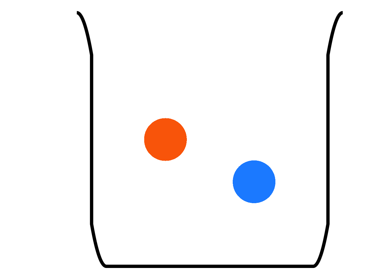
Figure 4.2: A Poorly-rendered Jar

Let’s say that we propose some defined experiments⁶⁴ regarding pulling a marble out of the jar (without peeking into the jar, of course). The first is what is the probability of drawing a blue marble out of the jar? Since there are two marbles in the jar, and, assuming that one draws one of them (I suppose one could reach in and miss both marbles and come out empty-handed, but let’s ignore that possibility for the purposes of this exercise), we may intuit that the probability of drawing one specific marble is $1/2$, or $0.5$, or $50%$.⁶⁵ More formally, we can define the sample space as:

\[\Omega=\{Blue, Orange\}\] since the probability of the sample space is 1 (thanks to the axiom of normalization) and the probability of either of these mutually exclusive events is the sum of the probabilities of each individual event (thanks to the axiom of finite additivity):

\[p(\Omega)=1 =p(Blue)+p(Orange)\] Assuming equal probability of each event (which is reasonable if we posit that there is no way to distinguish one marble from the other just be reaching into the jar without looking), then algebra so simple that we will leave out the steps tells us that:

\[p(Blue)=p(Orange)=\frac{1}{2}\] Thus, in this defined experiment, the probability of drawing a blue marble out of the jar in a singe draw is $1/2$.

Let’s define another experiment: we reach into the jar twice and pull out a single marble each time. Now, we have a defined experiment with two trials⁶⁶ What is the probability of drawing the blue marble twice? That probability depends on one important consideration: do we put the marble from the first draw back into the jar before drawing again? If the answer is yes, then the two trials are the same:

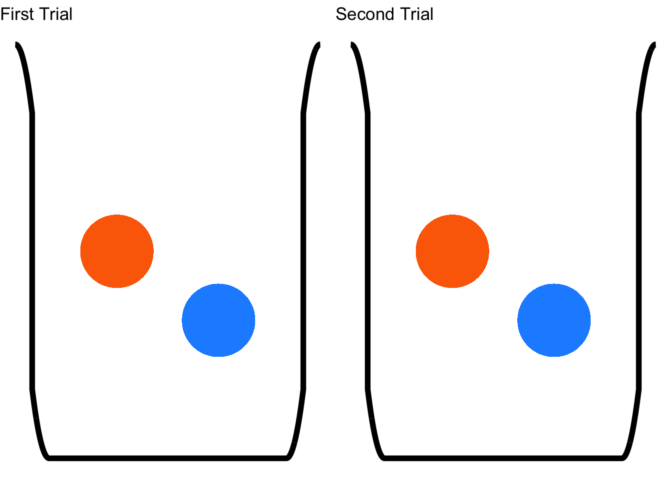
Figure 4.3: Sampling with Replacement

If we put whatever marble we draw on the first trial back into the jar before the second trial – or, in more formal terms, we sample with replacement⁶⁷ from the jar. That means that whatever event is observed in the first trial – whichever marble was chosen, in this example – has no effect on the probabilities of each event in the second trial – whichever marble is chosen second, in this example. If we put the first marble back in the jar, then the probability of choosing a blue marble on the second trial is the same as it was on the first trial and it does not matter which marble was selected in the first trial. The events drawing a marble in Trial 1 and drawing a marble in Trial 2 are therefore independent events⁶⁸ By definition, if events $A$ and $B$ are independent, then the probability of event $A$ happening given that event $B$ has occurred is exactly the same as the probability of event $A$ happening – since they are independent, the fact that $B$ may or may not have happened doesn’t matter at all for $A$ and vice versa:

\[A~and~B~are~independent~if~and~only~if~p(A|B)=p(A)~and~p(B|A)=p(B)\] ⁶⁹Now, we can modify the equation for determining the probability of $A\cap B$ for independent events:

\[if~p(B|A)=p(B), p(A\cap B)=p(A)p(B)\] And back to our marble example: if we are sampling with replacement, then we can call blue on the first draw event $A$ and blue on the second draw event $B$, the probability of each is $1/2$, and:

\[p(Blue_{trial~1}\cap~Blue_{trial~2})=p(Blue_{trial~1})p(Blue_{trial~2})=\left(\frac{1}{2}\right)\left(\frac{1}{2}\right)=\frac{1}{4}.\] Now let’s consider the other possible sampling method: what if we don’t put the first marble back in the jar? In that case, we have sampled without replacement⁷⁰, and the probabilities associated with events in the second trial depend on what happens in the first trial:

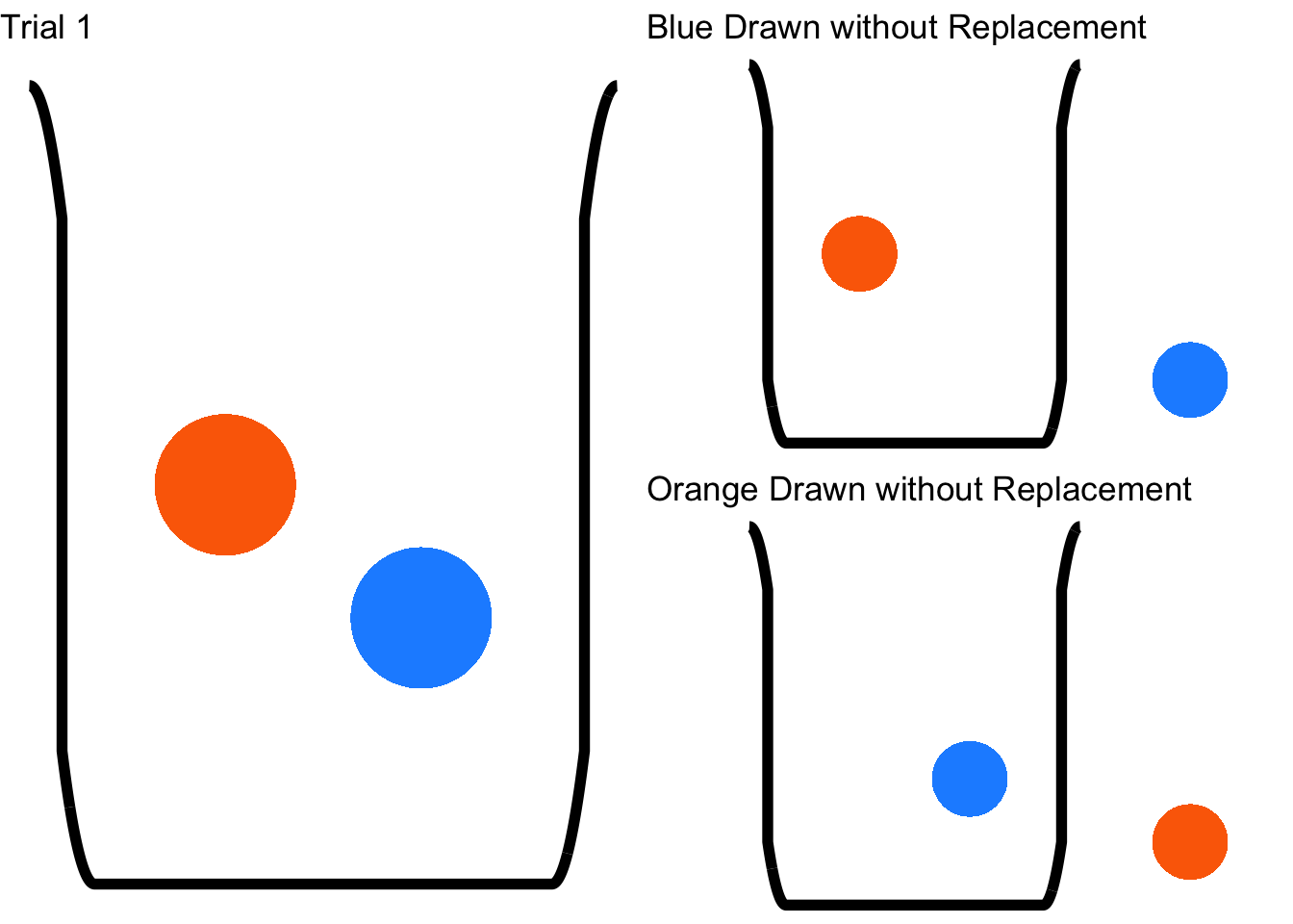
Figure 4.4: Sampling without Replacement

In this case, the probabilities of the events in Trial 2 are different given what happened in Trial 1 – they depend on what happened on Trial 1 – and thus are considered dependent events.⁷¹ In the case of dependent events, $p(A|B)\ne p(A)$ and $p(B|A)\ne p(B)$. So, based on the observed event in Trial 1, there are two possible sample spaces for Trial 2. If the blue marble is drawn on Trial 1 and not replaced, then on Trial 2:

\[\Omega=\{Orange\};~p(Blue_{Trial~2})=0,~p(Orange_{Trial~2})=1\] and if the orange marble is drawn in Trial 1 and not replaced, then on Trial 2⁷²:

\[\Omega=\{Blue\};~p(Blue_{Trial~2})=1,~p(Orange_{Trial~2})=0.\] So: what is the probability of drawing the blue marble twice without replacement? We can know – and Figure 4.4 can help illustrate – that it is impossible: if we take out the blue marble in Trial 1 and don’t put it back in, there is no way to draw a blue marble in Trial 2. The probability is 0. The math backs this up: the second draw depends on the result of the first draw, and the probability of drawing a blue marble in Trial 2 given that a blue marble was drawn in Trial 1 without replacement. Using the formula for and probabilities⁷³:

\[p(Blue_{trial~1}\cap~Blue_{trial~2})=p(Blue_{trial~1})p(Blue_{trial~2}|Blue_{trial~1})=\left(\frac{1}{2}\right)\left(0\right)=0.\]

4.4.1.1 Intersections of more than two events

The logic of intersection probability for two events holds for the intersection probabilities for more than two events, although the equations we use to evaluate them look more complex. The intersection probability of two events is given by the product of the probability of the first event and the probability of the second event given the first event. The intersection probability of three events is given by the product of the probability of the first event and the probability of the second event and the probability of the third event given the first event and the second event:

\[p(A\cap B\cap C)=p(A)p(B|A)p(C|A\cap B).\]

The intersection probability of four events is given by the product of the probability of the first event and the probability of the second event and the probability of the third event given the first event and the second event and the probability of the fourth event given the first event and the second event and the third event):

\[p(A\cap B\cap C \cap D)=p(A)p(B|A)p(C|A\cap B)p(D|A\cap B \cap C)\]

and so on. Please note that the names that we give to events – $A$, $B$, $C$, etc. – are arbitrary. When assessing the probability of multiple events, we can give any letter name to any event and our designations by themselves are not that important. What is important is understanding which events depend on which. It’s helpful to use letter labels to write out equations in a general sense, but when doing actual problems, I recommend using more descriptive labels (as in: full or abbreviated names of the events themselves) so that it’s easier to keep track of the relationships between the events.

To help us understand the intersection of more than two events, first let’s look at a case where all of the events are independent of each other. In this example there are four events: $A$, $B$, $C$, and $D$. Because all of the events are independent of each other, then by the definition of independent events: $p(B|A)=p(B)$, $p(C|A\cap B)=p(C)$, and $p(D|A\cap B \cap C)=p(D)$. Thus, the equation for the intersection probability of these events simplifies to:⁷⁴

\[p(A\cap B\cap C\cap D)=p(A)p(B)p(C)p(D)\]

This example is a personal favorite of mine, because I think it links a somewhat complex intersection probability with a more intuitive understanding of probability as $x$ chances in $y$. It’s about gambling. ⁷⁵ Specifically, it’s about one of the lottery games run by the Commonwealth of Massachusetts: The Numbers Game. In that game, there are four spinning wheels (pictured in Figure 4.5), each with 10 slots representing each digit from 0 – 9 one time, and there is a ball placed in each wheel. The wheels spin for a period of time, and when they stop spinning, the ball in each wheel comes to rest on one of the digits.

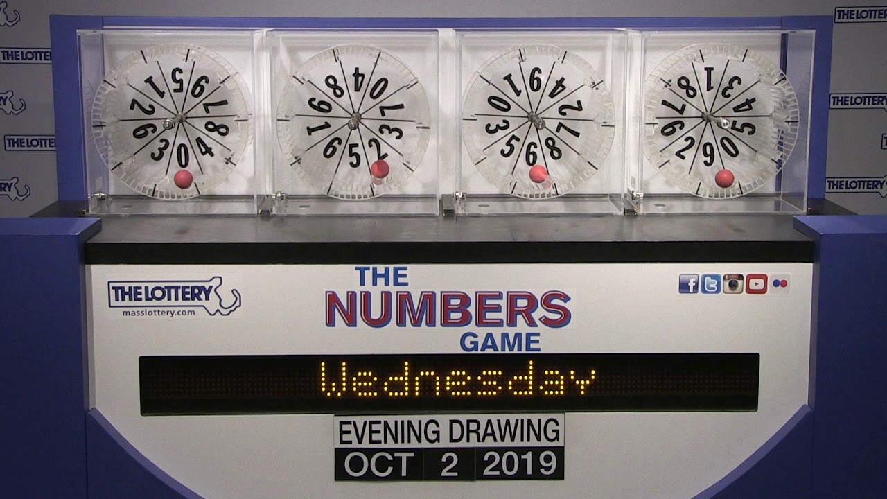
Figure 4.5: The Massachusetts Lottery Numbers Game, known in Boston-area locales as THE NUMBAH

The result is a four-digit number, and to win the jackpot, one has to pick all four digits in the correct order. ⁷⁶ Each wheel is equally likely to land on each of the 10 digits (0 – 9), and each wheel spins independently so that the outcome on each wheel is literally independent of the outcomes on any of the other wheels. Thus, the probability of picking the correct four digits in order is the intersection probability of picking each digit correctly. In other words: it’s the probability of picking the first digit correctly and picking the second digit correctly and picking the third digit correctly and picking the fourth digit correctly:

\[p(jackpot)=p(1st~digit~\cup 2nd~digit~\cup 3rd~digit~\cup 4th~digit).\] Since we know that each digit is an independent event, we need not concern ourselves with conditional probabilities: the probability any digit is $1/10$, and is exactly the same regardless of any of the other digits (symbolically: $p(2nd~digit)=p(2nd~digit|1st~digit)$, $p(3rd~digit)=p(3rd ~digit|1st~digit\cap 2nd~digit)$, and $p(4th~digit)=p(4th~digit|1st~digit\cap 2nd~digit\cap 3rd~digit)$). So, the probability of the jackpot is:

\[p(jackpot)=p(1st~digit)p(2nd~digit)p(3rd~digit)p(4th~digit)\]

\[=\left( \frac{1}{10} \right) \left( \frac{1}{10} \right) \left( \frac{1}{10} \right) \left( \frac{1}{10} \right)=\frac{1}{10000}.\] Thus, the probability of picking the winning series of numbers is $1/10000$: if you bought a ticket for the numbers $8334$, then there’s a $1/10000$ probability that that set of numbers comes up; if you bought a ticket for the numbers $5782$, there’s a $1/10000$ chance that that number wins as well.⁷⁷ Which brings us to the reason why I like this example so much: the combinations of digits in the numbers game perfectly resemble four-digit numbers (although sometimes they have leading zeroes). The possible combinations of digits in the game go from $0000$ to $9999$. How many integers exist between 0 and 9,999, 0 included? Exactly as many numbers as between 1 and 10,000: 10,000. If, instead of asking you to wager on four digits in a particular order, you were asked to pick a number between 0 and 9,999, what would your probability be of choosing the right one? It would be $1/10000$ – the same result as we got above. Which is nice.

Another fun feature of using The Numbers Game as an example is that since each of the wheels is the same, spinning all of the wheels at the same time gives the same expected outcomes that spinning one of the wheels four times would do – it would just take longer to spin one four times – so effectively it’s an example of sampling with replacement.

Now let’s examine how intersections of more than two events work when events are dependent with an example of sampling without replacement. For this example, we’ll talk about playing cards again. Let’s say that you are dealt four (and only four) cards from a well-shuffled deck of ordinary playing cards.⁷⁸ What is the probability that you are dealt four aces? Please note: since you are being dealt these cards, they are not going back into the deck: this is sampling without replacement.

There are four aces in a deck of 52 playing cards, so the probability of being dealt an ace on the first draw is $4/52$. If you are dealt an ace on the first draw (if you aren’t dealt an ace on the first draw, the probability of getting four aces in four cards is zero so that doesn’t matter), then there will be three aces left in a deck of 51 cards, so the probability of being dealt an ace on the second draw will be $3/51$. If you are dealt aces on each of the first two draws, then there will be two aces left in a deck of 50 cards, so the probability of being dealt a third ace will be $2/50$. Finally, if you are lucky enough to be dealt aces on each of the first three draws, then there will be one ace left in a deck of 49 cards, so the probability of being dealt a fourth ace will be $1/49$. We can express that whole last paragraph in math-symbol terms like:

\[p(Ace_{first})=\frac{4}{52}\] \[p(Ace_{second}|Ace_{first})=\frac{3}{51}\] \[p(Ace_{third}|Ace_{first}\cap Ace_{second})=\frac{2}{50}\]

\[p(Ace_{fourth}|Ace_{first}\cap Ace_{second} \cap Ace_{third})=\frac{1}{49}\]

Being dealt four aces out of four cards is equivalent to saying being dealt an ace on the first draw and being dealt an ace on the second draw and being dealt an ace on the third draw and being dealt an ace on the fourth draw: it’s the intersection probability of those four related events. Using the equation $p(A\cap B \cap C \cap D)=p(A)p(B|A)p(C|A\cap B)p(D|A\cap B \cap C \cap D)$ and substituting the probabilities of each Ace-drawing event outlined above, the probability of four consecutive aces from a well-shuffled 52-card deck is:

\[p(4~Aces)=\left( \frac{4}{52} \right) \left( \frac{3}{51} \right) \left( \frac{2}{50} \right) \left( \frac{1}{49} \right) =\frac{24}{6497400}\approx0.00000369\]

which is a very small number. Drawing four consecutive aces is not very likely to happen. And yet: it’s exactly as likely as drawing four consecutive jacks or four consecutive 9’s, and 24 times more likely than the combination of any four specific cards (like, the queen of spades and the five of hearts] and the 10 of clubs and the 2 of diamonds ⁷⁹

I noted above that keeping track of which events may depend on others is important (far more important than which event you call $A$ and which event your call $B$). The examples of the lottery game (independent events) and of dealing aces (dependent events) are relatively simple ones. It can get extremely complicated to keep track of not only what depends on what but also the ways in which those dependencies change sample spaces – that is: what the probability of one event is given other events. Probability trees are visualizations of relationships between events that I find very helpful for both keeping track of things and for calculating complex probabilities, and we will get to those, but first, we need to talk about unions

4.4.2 Unions

The total occurrences of events, e.g., event $A$ or event $B$ happening, is known as the union⁸⁰ The probability of event $A$ or event $B$ happening is thus equivalently expressed as the union probability of $A$ and $B$, as $p(A)\cup~p(B)$, and as $p(A\cup B)$.

We know already from the finite additivity axiom of probability that the total probability of mutually exclusive events is the sum of of the probabilities of each of the events. Now that we are more familiar with terminology and symbology, we can write that axiom as:

\[if~p(A\cap B)=0,~p(A\cup B)=p(A)+p(B)\] where the term $p(A\cap B)=0$ represents the condition of $A$ and $B$ being mutually exclusive (and thus the probability of $A$ and $B$ both happening being 0).

You may have be wondering, “what happens if the events are not mutually exclusive?” and even if you are not wondering that, I will tell you anyway. Let’s say we are interested in the combined probability of two events $A$ and $B$ that can co-occur – for example, the probability that, in two flips of a fair coin, the coin will turn up heads both times. In that example, the coin could turn up heads on the first flip and turn up heads on the second flip and turn up heads on both flips. If we incorrectly treated the events $Heads_{flip 1}$ and $Heads_{flip 2}$ as independent events, we would incorrectly conclude that the probability of observing heads on either of two flips is $p(Heads_{flip~1})+p(Heads_{flip~2})=0.5+0.5=1$. That conclusion, in addition to being wrong, doesn’t make sense: it obviously is possible to observe 0 heads in two flips of a fair coin. If we want to get even more absurd about it, we can imagine three flips of a fair coin: surely the probability of three consecutive heads is not $p(Heads_{flip~1})+p(Heads_{flip~2})+p(Heads_{flip~3})$ because that would be $0.5+0.5+0.5=1.5$ and thus violate the axiom of Normalization.

What is causing that madness of seemingly overinflated union probabilities? The union probability of $A$ and $B$ can be thought of as the probability of $A$ or $B$, but it can also be considered the total probability of $A$ and $B$, which means that it’s the probability of:

$A$ happening and $B$ not happening ($A \cup \neg B$),
$B$ happening and $A$ not happening ($B \cup \neg A$), and
$A$ and $B$ happening ($A \cup B$).

When we add the probabilities of events that are not mutually exclusive, we are effectively double-counting the probability of $A \cup B$. Consider the following problem: two people – Alice and Bambadjan (conveniently for the math notation we have been using, we can call them $A$ and $B$) – have consistent and different sleep schedules. Alice goes to sleep every night at 10 pm and wakes up at every morning at 6 am. Bambadjan goes to sleep every night at 4 am and wakes up every day at 12 pm. During any given 24-hour period, what is the probability that Alice is asleep or Bambadjan is asleep?

The probability of the co-occurrence of two events – whether the events are mutually exclusive are not – is given by the equation:

\[p(A\cup B)=p(A)+p(B)-p(A\cap B)\]

Let’s visualize what this equation means by representing the sleep schedules of Alice ($A$) and Bamnadjan ($B$) as timelines:

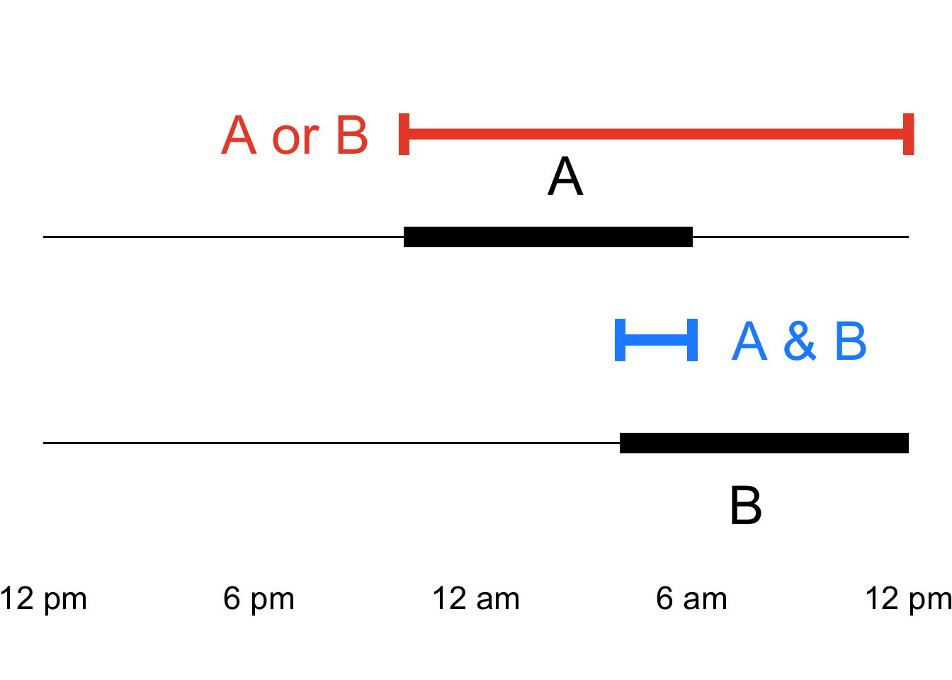
Figure 4.6: The Sleep Schedules of Alice and Bambadjan

Hopefully, the figure makes it easy to see that if we are interested in the times that either Alice or Bambadjan is asleep, then then the time when their sleep overlaps does not matter. More than that: that overlap will mess up our calculations. If we add up the times that A. Alice is asleep, B. Bambadjan is asleep, and C. both Alice and Bambadjan are asleep, we get \[8~hours+8~hours+2~hours=18~hours.\] If you add to that result to the 10 hours per day when neither Alice nor Bambadjan is asleep (between 12 pm and 10 pm), you get a 28-hour day, which is not possible on Planet Earth.

Figure 4.7: only 24 hours per day here

So, we have to account for the double-counting of the time when both are asleep – the intersection of event $A$ (Alice being asleep) and event $B$ (Bambadjan being asleep). Using the above equation for intersection probabilities for non-exclusive events:

\[p(A\cup B)=p(A)+p(B)-p(A\cap B)=\frac{8}{24}+\frac{8}{24}-\frac{2}{24}=\frac{14}{24}\]

4.4.2.1 Unions of More than Two Events

When two events are mutually exclusive, calculating their union probability is simple: since there is no intersection probability of the two events, the intersection term of the equation drops out and we are left with $p(A\cup B)=p(A)+p(B)$. That simplicity holds when calculating the union probability of more than two mutually exclusive events:

\[if~p(A\cap B)=p(A \cap C) = p(B \cap C) = p(A\cap B \cap C)=0,~then\] \[p(A\cup B \cup C)=p(A)+p(B)+p(C).\]

For example, let’s consider the probability of a person’s birthday falling on one day or another. Assuming that the probability of having a birthday on any one given day of the week is $1/7$,⁸¹ what is the probability that a person’s birthday falls on a Monday or on a Wednesday or on a Friday? These three events (1. birthday on Monday, 2. birthday on Wednesday, 3. birthday on Friday) are mutually exclusive, so, the calculation for that probability is straightforward:

\[p(Monday \cup Tuesday \cup Wednesday)=\frac{1}{7} + \frac{1}{7} + \frac{1}{7} =\frac{3}{7}\] And, of course, the probability that a person’s birthday falls on any day of the week is $1/7+1/7+1/7+1/7+1/7+1/7+1/7=1.$

As you might imagine, the union probabilities of more than two events when some or all are not mutually exclusive is a bit more difficult. Here is a diagram representing the union probability of two intersecting events; it is similar to the one we used to examine the union probability of Alice and Bambadjan being asleep, but a little more generic:

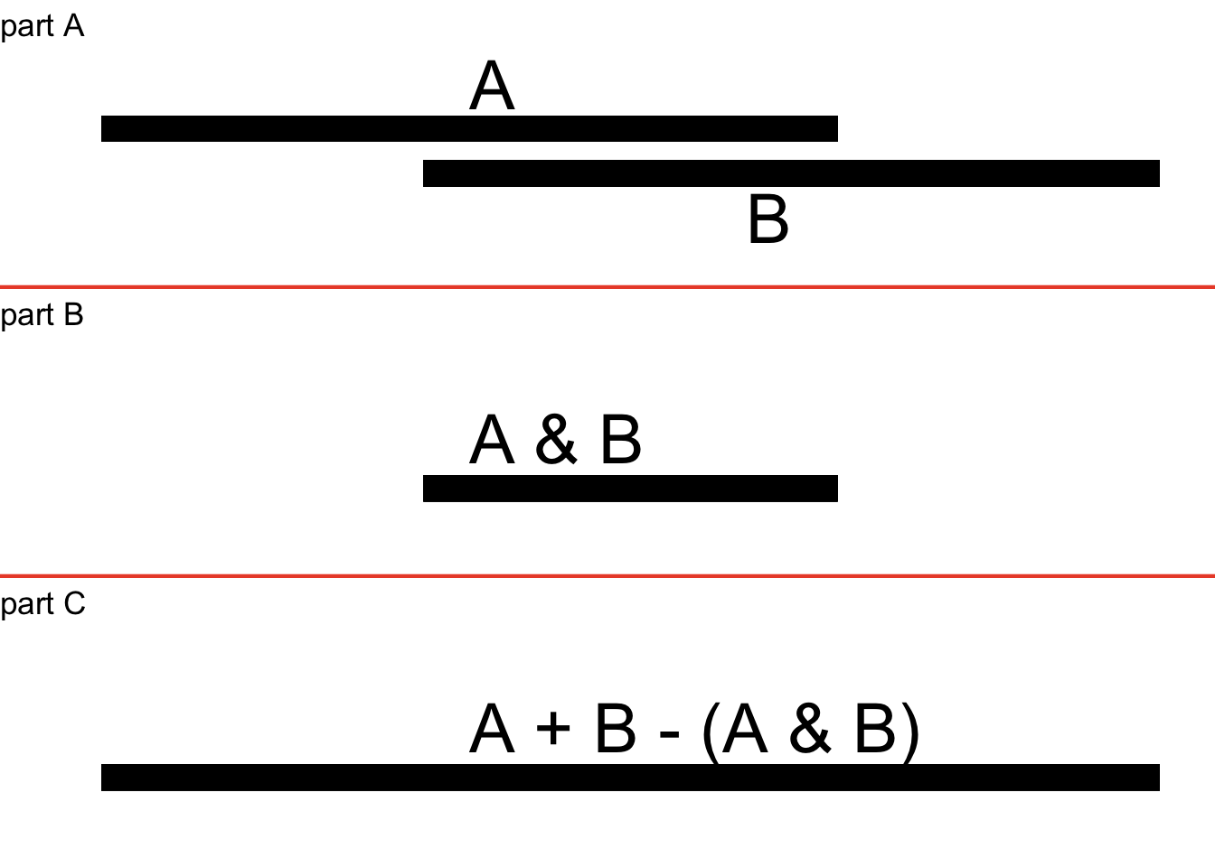
Figure 4.8: Generic Representation of Union Probability of Two Intersecting Events

As we can see in Figure 4.8, when we add up the occurrence of two intersecting events (part A), we double-count the intersection (part B), so we have to subtract the intersection from the sum to get the union of two events (part C).

In Figure 4.9, we add a third intersecting event $C$ to intersecting events $A$ and $B$. The range of outcomes for the three events separately are represented in part A, and the four intersections between the events – $A \cup B$, $A \cup C$, $B \cup C$, and $A \cup B \cup C$ – are shown in Figure 4.9, part B.

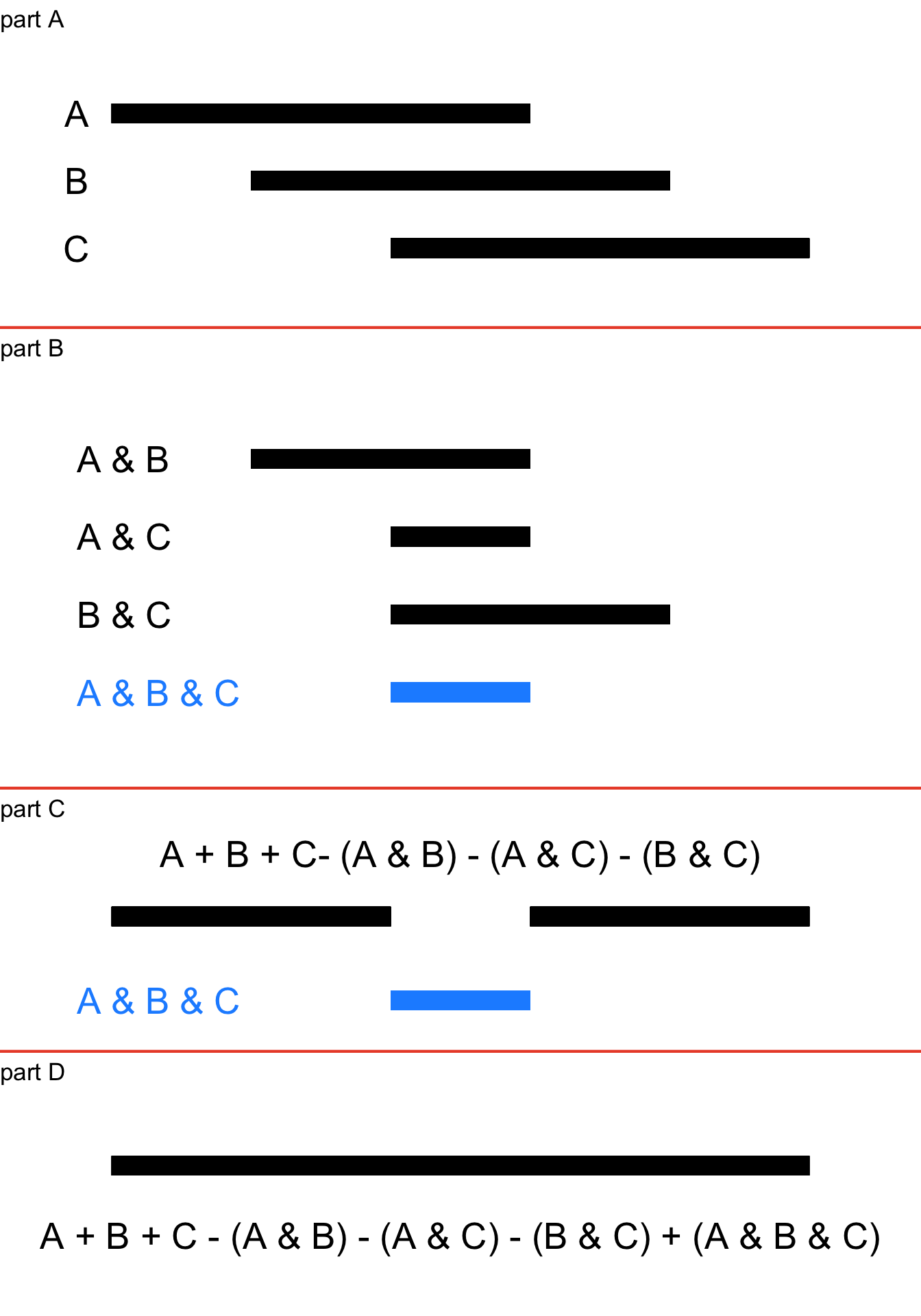
Figure 4.9: Generic Representation of Union Probability of Three Intersecting Events

In Figure 4.9, part C, we see what happens when we add up the events and subtract the pairwise intersections $A\cap B$, $B\cap C$, and $A\cap C$: we end up under-counting the three-way intersection $A\cap B \cap C$. That happens because the sum of $A$ and $B$ and $C$ has two areas of overlap in the $A\cap B \cap C$ section (that is, in that area, you only need one of the three but you have three, so, two are extra) and when we subtract the three pairwise intersections from the sum – which we have to do to account for the double-counting between pairs of events – we take three away from that section, leaving it empty. Thus, we have to add the three-way intersection (the blue line in part C) back in to get the whole union probability shown in part D.

Thus, the general equation for the union probability of three events is:

\[p(A\cup B \cup C)=\] \[p(A)+p(B)+p(C)\] \[-p(A\cap B)-p(A\cap C)-p(B \cap C)\] \[+p(A\cap B\cap C)\] and⁸² for any combinations of those events that are mutually exclusive, the interaction term for those combinations is 0 and drop out of the equation.

Just like knowing which events depend on which other events and how in calculating intersection probabilities can be tricky, keeping track of which events intersect with each other and how in calculating union probabilities can also be tricky, and keeping track of all of those things at the same time can be multiplicatively tricky. In the next section, we will talk about a visual aid that can help with all of that trickiness.

4.5 Expected Value and Variance

The terms Expected Value and Variance were introduced in the page on categorizing and summarizing information. Both terms apply to general probability theory as well.

The expected value of a defined experiment is the long-term average outcome of that experiment over multiple iterations. It is calculated as the mean outcome weighted by the probability of the possible outcomes. If $x_i$ is the value of each event $i$ among $N$ possible outcomes in the sample space, then:

\[E(x)=\sum_{i=1}^N x_i p(x_i)\]

For example, consider a roll of a six-sided die. The sample space for such a roll is $\Omega=\{1, 2, 3, 4, 5, 6\}$: thus, $x_1=1$, $x_2=2$, $x_3=3$, $x_4=4$, $x_5=5$, and $x_6=6$. The probability of each event is $1/6$, so $p(x_1)=p(x_2)=p(x_3)=p(x_4)=p(x_5)=p(x_6)=1/6$. The expected value of a roll of a six-sided die is therefore:

\[E(x)=1\left( \frac{1}{6} \right)+2\left( \frac{1}{6} \right)+3\left( \frac{1}{6} \right)+4\left( \frac{1}{6} \right)+5\left( \frac{1}{6} \right)+6\left( \frac{1}{6} \right)=\frac{21}{6}=3.5.\] Note that you can never roll a 3.5 with a six-sided die! But, in the long run, that’s on average what you can expect.

Next, let’s consider a roll of two six-sided die. Each die has a sample space of $\Omega=\{1, 2, 3, 4, 5, 6\}$, so the sample space of the two dice combined is:

	Die 2
Die 1	1	2	3	4	5	6
1	2	3	4	5	6	7
2	3	4	5	6	7	8
3	4	5	6	7	8	9
4	5	6	7	8	9	10
5	6	7	8	9	10	11
6	7	8	9	10	11	12

The expected value of a roll of two six-sided dice is the sum of the values in the table (it’s 252) divided by the total number of possible outcomes (36), or 7.

We could also arrive at the same number by defining the sample space as $\Omega=\{2, 3, 4, 5, 6, 7, 8, 9, 10, 11, 12\}$, and noting that there are more ways to arrive at some of those values than others. The number 7, for example, can happen 6 different ways, and so $p(7)=6/36=1/6$⁸³ Multiplying each possible sum of the two dice by their respective probabilities gives us:

\[E(x)=2\left(\frac{1}{36}\right)+3\left(\frac{2}{36}\right)+...+12\left(\frac{1}{36}\right)=\frac{252}{36}=7.\] The variance of a defined experiment is given by:

\[V(x)=\sum_{i=1}^N\left(x_i-E(x)\right)^2p(x_i)\] which is a way to describe the range of possible outcomes in a defined experiment.

4.5.1 Probability Trees

Probability Trees, also known as Tree Diagrams, are visual representations of the structure of probabilistic events. There are three elements to a probability tree:⁸⁴

Node: a point on the diagram indicating a trial.
Branch: the connection between nodes and events; we indicate on branches the probability of the events for a given trial.
Event (or Outcome): an event (or outcome). Given that we’ve already defined event (or outcome), this definition is pretty straightforward and a little anticlimactic.

Figure 4.10 is a probability tree for a single flip of a fair coin with labels for the one node, the two branches, and the two possible outcomes of this trial.

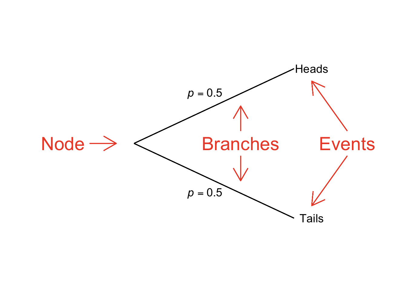
Figure 4.10: Probability Tree Depicting One Flip of a Fair Coin

We can think of the node as a starting point for the probabilistic paths that lead to events, with the probability of taking each path written right on the branches. In the case of a coin flip, once the coin is flipped (the node), we can see from the diagram that there is a probability of 0.5 that we will take the path to heads and a probability of 0.5 that we will take the path that ends in tails. Using a tree diagram to map out the probabilities associated with a single coin flip is perfectly legitimate, but not terribly necessary – it’s a pretty simple example. Probability trees can be – and usually are – more complex (but tend to be less complex than algebraic representations of the same problems, otherwise, that would defeat the point of using a tree to help us understand the math). A node can take on any number of branches, and each event can, in turn, serve as a node for other branches and events. For example, in Figure 4.11, we have a probability tree representation of two flips of a fair coin.

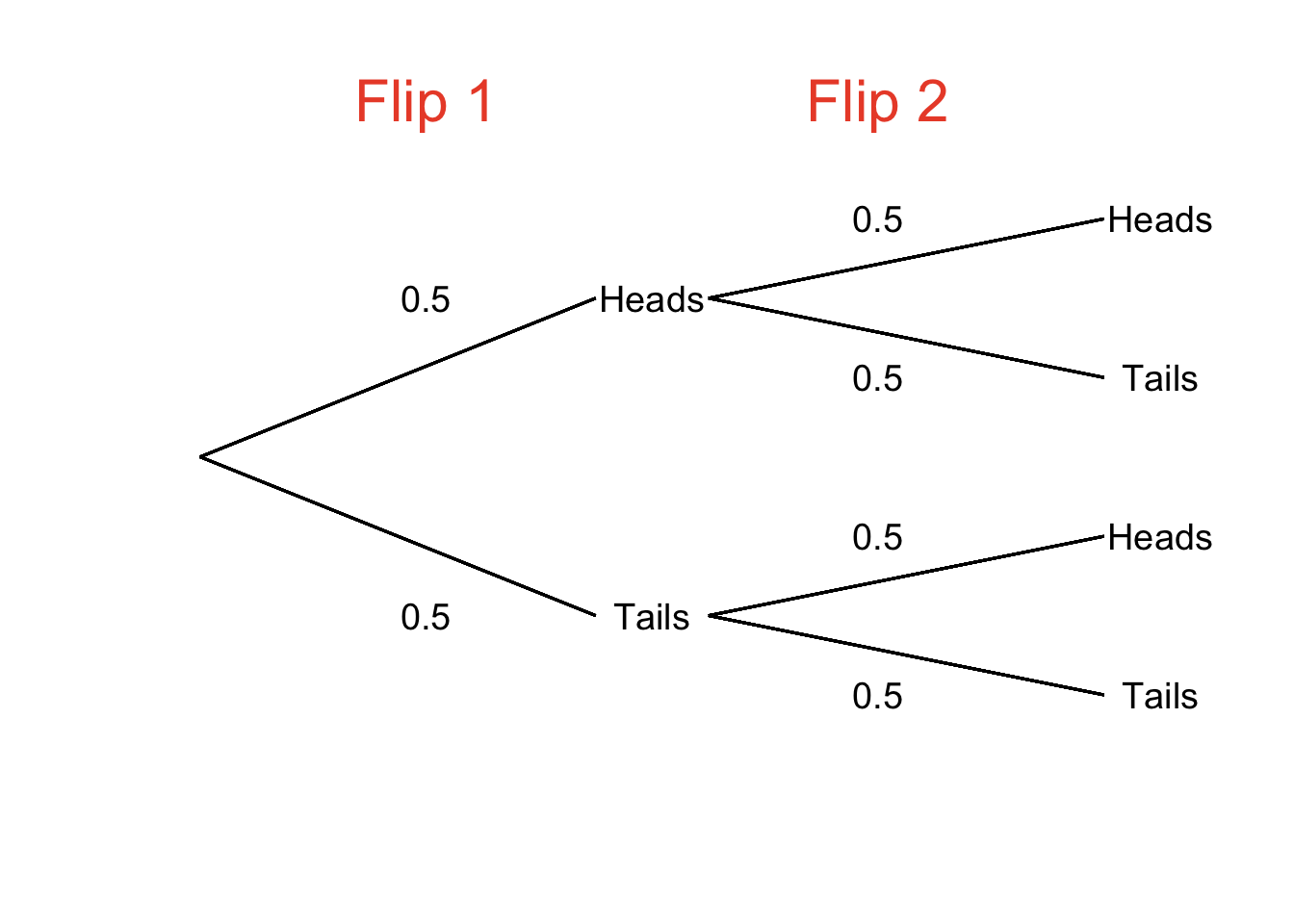
Figure 4.11: Probability Tree Depicting Two Flips of a Fair Coin

Connected branches represent intersections. In Figure 4.11, the path that goes from the first node to Heads and then continues on to Heads again represents the probability $p(Heads_{flip~1} \cap Heads_{flip~2})$. The sum of probabilities of events are unions. The event of getting exactly one heads and one tails in two flips is represented in two ways in Figure 4.11: one could get heads first and then tails or get tails first and then heads. We can also see from the diagram that these events are mutually exclusive (on neither flip can you get heads and tails), so, the probability of one heads and one tails in two flips is the sum of the intersection probabilities $p(Heads_{flip~1} \cap Tails_{flip~2})$ and $p(Tails_{flip~1} \cap Heads_{flip~2})$:

\[p(1~Heads,~1~Tails)=p(Heads_{flip~1}\cap Tails_{flip~2}\cup Tails_{flip~1}\cap Heads_{flip~2})=(0.5)(0.5)+(0.5)(0.5)=0.5.\]

In general, then, the rule for working with probability trees is multiply across, add down.

The probabilities on the branches of tree diagrams can take on any possible probability value and therefore can be adjusted to reflect conditional probabilities. For example: let’s say there is a jar with 3 marbles in it: 1 red marble, 1 yellow marble, and 1 green marble. If, without looking into the jar, we took one marble out at a time without replacement, then the probability of drawing each marble on each draw would be represented by the tree diagram in Figure 4.12.

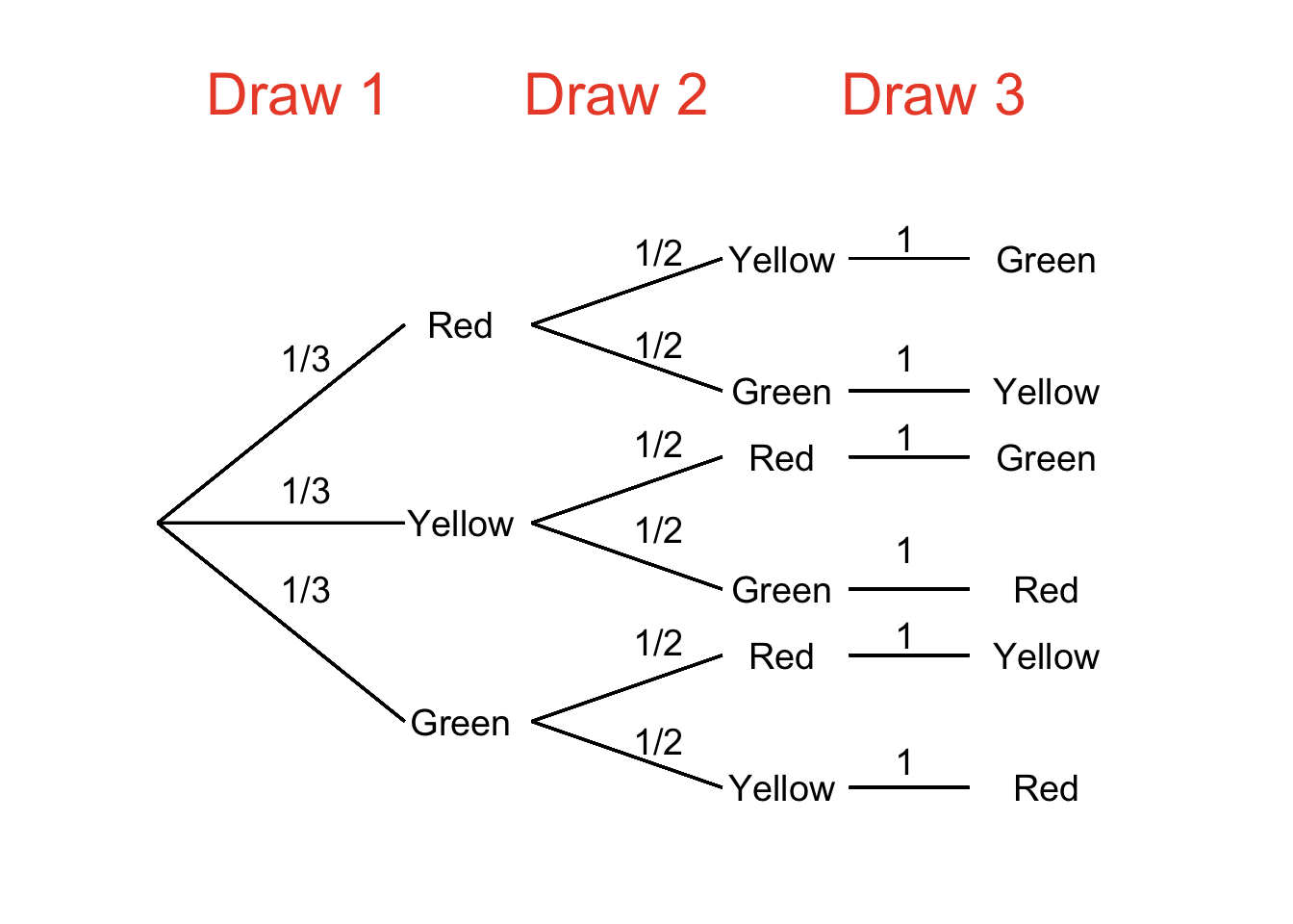
Figure 4.12: Probability Tree Depicting Sampling Without Replacement

We can use the diagram in Figure 4.12 to answer any probability questions we have about pulling marbles out of the jar. What is the probability of pulling out marbles in the order Red, Yellow, Green? We can follow the topmost path to find out: the probability of drawing Red first is $1/3$. Given that we have drawn Red first, the probability of drawing Yellow next is $1/2$. Finally, given that Red and Yellow have been drawn, the probability of drawing Green on the third draw is 1. Multiplying across the path (as we do), the probability of drawing marbles in the order Red, Yellow, Green is $(1/3)(1/2)(1)=1/6$. What is the probability of drawing Yellow last? That is given by adding the products of the two paths that end in Yellow: adding down (as we do), the probability is $(1/3)(1/2)(1)+(1/3)(1/2)(1)=2/6=1/3$. We can use the tree to examine probabilities before the terminal events as well. For example: what is the probability of drawing Green on the first or second draw? We can take the probability of Green on draw 1 – $1/3$ – and add the probabilities of drawing Red on the first draw and Green on the second draw – $(1/3)(1/2)=1/6$ and of drawing Yellow first and Green second – also $(1/3)(1/2)=1/6$ and we get $(1/3)+(1/6)+(1/6)=4/6=2/3$.

4.6 Elementary and Compound (or Composite) Events

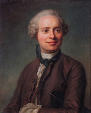
Figure 4.13: Jean-Baptiste le Rond d’Alembert.

Jean d’Alembert (1717 – 1783) was a French philosophe and mathematician. He was a co-editor (with Denis Diderot) of the Encyclopedia and contributed to it over a thousand articles, one of which was Heads or Tails, an essay about games of chance. In that article, he gives a sophisticated and ahead-of-its-time analysis of The St. Petersburg Paradox, one of the critical probability problems in the field of behavioral economics. However, that article isn’t known for that at all. It’s known for one of the most famous errors in probabilistic reasoning ever made by a big-deal mathematician in print.

Here’s why d’Alembert gets d’unked on. Say we’re playing a coin-flipping game (imagine it’s mid-18th-century France and this is the kind of thing we do for fun) where I flip a coin twice and you win if it comes up heads on either flip. d’Alembert argued that if you got heads on the first flip then the game would stop there, thus, there were three possible outcomes of the game: heads on the first flip (and no second flip), tails on the first flip and heads on the second flip, and tails on the first flip and tails on the second flip. In sample-space terms, d’Alembert was describing the game as $\Omega=\{H,~TH,~TT\}$ and – here’s the big problem – said that each of those outcomes was equally probable ($p=1/3$ each). We can pretty easily show why that conclusion is wrong (and we can refer to Figure 4.11 – to help): the probability of getting heads on the first flip is $1/2$ regardless of what happens after that flip,⁸⁵ and the probability of both heads after tails and tails and tails is $1/4$.

I bring d’Alembert’s error up for two reasons:

I find it comforting to know that a historically great mathematician can make mistakes, too, and I hope you do as well, and
Without meaning to, d’Alembert’s calculation conflated elementary events⁸⁶ and composite (or compound) events⁸⁷

An elementary event is an event that can only happen in one specific way. If I were to ask what is the probability that I (Dan, the person writing this right now) will win the gold medal in men’s singles figure skating at the next Winter Olympics?, then I would be asking about the probability of an elementary event: there is only one me, that is only one Olympic sport, and there is only one next Winter Olympics. Also, that probability would be 0, but that’s beside the point (If it weren’t for the axiom of nonnegativity, the probability of me winning a skating competition would be negative – I can barely stand up on skates). If I were to ask what is the probability that an American wins the gold medal in men’s figure skating at the next Winter Olympics, I would be asking about the probability of a composite event: there are multiple ways that could happen because there are multiple men in America, each of whom represents a possible elementary event of winning the gold in that particular sport in that particular Olympics.

Back to our man d’Alembert and the problem of two coin flips: in two flips of a fair coin, we might say that there are three possible outcomes:

Two heads (and zero tails)
One heads (and one tails)
Zero heads (and two tails)

And we can describe the sample space as:

\[\Omega =\{2H,~1H,~0H\}\] That’s all technically true, but misleading, because one of those outcomes is composite while the other two are elementary. That is: there are two ways to get one heads in two flips: you can get heads then tails or you can get tails then heads. There is only one way to get two heads – you must get heads then heads again – and there is only one way to get zero heads – you must get tails then tails again – so there are twice as many ways to get one heads than two get either two heads or zero heads.

Thus, a better, less misleading way to characterize the outcomes and the sample space of two coin flips is to do so in terms of the four elementary outcomes:

heads on flip one and heads on flip two
heads on flip one and tails on flip two
tails on flip one and heads on flip two
tails on flip one and tails on flip two

\[\Omega =\{HH,~HT,~TH,~TT\}\] The probability of each of those elementary events is equal⁸⁸ and by breaking down events into their elementary components, we avoid making the same mistake as d’Alembert did.

4.7 Permutations and Combinations

As we saw in the previous section on elementary and compound events, defining sample spaces is really important for properly understanding the probabilities involved with a given set of events. In relatively simple defined experiments like two flips of a fair coin or pulling a green marble out of a jar or drawing a card from a deck, the sample spaces are straightforward to define. When there are lots more possibilities and contingencies between those possibilities, defining the sample space can be much trickier. In this section, we are going to talk about two such situations and the mathematical tools we have to make those tricky tasks a lot simpler.

4.7.1 Permutations

Here’s an example to describe what we’re talking about with complex sample spaces: imagine five people are standing in a line.

Figure 4.14: Pictured: Five People Standing in Line in a Stock Photo that I did not Care to Pay For.

How many different ways can those five people arrange themselves? Let’s start with the front of the line. There are five options for who stands in the first position. One of those five goes to the front of the line, and now there are four people left who could stand in the second position. One of those four goes behind the first person, and then there are three left for the third position, then there will be two left for the fourth position, and finally there will be only one person available for the end of the line.

Let’s call the people $A$, $B$, $C$, $D$, and $E$, which would be rude to do in real life but they’re fictional so they don’t have feelings. For each of the five possible people to stand in the front of the line, there are four possibilities for people to stand behind them:


If	$A$	is in the first position, then	$B \cup C \cup D \cup E$	can be in the second position
	$B$		$A \cup C \cup D \cup E$
	$C$		$A \cup B \cup D \cup E$
	$D$		$A \cup B \cup C \cup E$
	$E$		$A \cup B \cup C \cup D$

That’s $5\times 4=20$ possibilities of two people in the first two parts of the line. For each of those 20 possibilities, there are three possible people that could go in the third position, so for the first three positions we have $5\times 4 \times 3 = 60$ possibilities. The pattern continues: for the first four positions we have $5\times 4 \times 3 \times 2 = 120$ possibilities, and for each of those 120 possibilities there is only one person left to add at the end so we end up with a total of $5\times 4 \times 3 \times 2 \times 1= 120$ possibilities for the order of five people standing in a line.

In general, the number of possible orders of $n$ things is, as in our example of five people standing in a line, $n\times (n-1) \times (n-2) \times ... \times 1)$. That expression is equivalent to the factorial of $n$, symbolized as $n!$.⁸⁹ In our example, there were $n=5$ people standing in line so there were $5!=120$ possible orders. If you had two items to put on a shelf, there would be $2!=2$ ways to arrange them; if you had six items to put on a shelf, there would be $6!=720$ ways to arrange them.

Now let’s say that we had our same five people from above but only three could get in the line. How many ways could three people selected out of the five people stand in order? The math starts out the same: there are five possibilities for the first position, and four possibilities for the second for each of the five in the first, and three possibilities for each of the five in the first and four in the second: $5 \times 4 \times 3 = 60$ possibilities. What happens next? Nothing. There are no more spots in the line, so whomever is left out doesn’t get a spot in the line (which could be sad, but again: fictional people don’t have emotions so don’t feel too bad for them).

At this point – and this may be overdue – we can define the term permutation.⁹⁰ Permutations are combinations of things where the order of those things matters. The term includes orders of $n$ objects, but also combinations of fewer than $n$ of those objects with order.

Note what happened when we removed two possible positions from the line where five people were to stand. We took the calculation of the number of possible orders – $5!=5\times 4\times 3\times 2\times 1=120$ – and we removed the last two terms (because we ran out of room in the line). We didn’t subtract them, but rather, we canceled them out. To do that mathematically, we use division:

\[60=\frac{5\times 4\times 3\times 2\times 1}{2\times 1}=5\times 4\times3\]
which is equivalent to:

\[60=\frac{5!}{2!}.\]

Let’s briefly look at another example: imagine you had 100 items and you had a small shelf with space for only two of those items; how many different ways could that shelf look? For the first spot on the shelf, you would have 100 options. For the second spot, whatever choice you made for the first spot would leave 99 possibilities for the second spot. And then you would be out of shelf space, so the total number of options would be $100\times 99=9,900$. Another way to think of that is that from the $100!$ possible orders of all of your items, you canceled out the last $100-2=98$ possibilities:

\[9,990=100\times 99=\frac{100!}{98!}\] In general, then, we can say that the number of permutations of $n$ things given that they will be put in groups of size $r$ – or as we officially say it, n things Permuted r at a time – and as we symbolically write it $_nP_r$ – is:

\[nPr=\frac{n!}{(n-r)!}\]

That equation works just as well when $r$ – the number of things being permuted at a time – is the same as $n$ – the number of things available to permute. In our original example, we had five people to arrange themselves in a line of five. The number of permutations is given in that case by:

\[_5P_5=\frac{5!}{(5-5)!}=\frac{5!}{1}=120\] keeping in mind the fact noted in the sidenote above and in the bonus content below that the factorial of 0 is 1.

4.7.2 Combinations

Permutations are arrangements of things for which the order matters. When things are arranged in ways and the order doesn’t matter, those arrangements are called combinations.⁹¹ Above, we calculated the number of possible permutations for five people standing in a line: $_5P_5=5!/0!=120.$ But what if order doesn’t matter – what if it’s just five people, standing not in a line, but just scattered around? How many ways can you have a combination of five people given that you started with five people? Just one. If their relative positions don’t matter, there’s only one way to combine five people in a group of five. The number of combinations is always reduced by a factor of the number of possible orders relative to the number of permutations. As mentioned in the previous section, the number of orders is the factorial of the number of things in the group: $r!$. Thus, we multiply the permutation formula by $1/r!$, putting $r!$ in the denominator, to get the combination formula for n things Combined r at a time (also known as the combinatorial formula):

\[nCr=\frac{n!}{(n-r)!r!}\]

Thus, while there are $5!/0!=120$ possible permutations of five people grouped five at a time, there is just $5!/(5!1!)=1$ possible combination of five people grouped five at a time.

Here’s another example: imagine that you are going on a trip and you have five books that you are meaning to read but you can only bring three in your bag. How many combinations of three books can you bring?⁹² The order of the books doesn’t matter, so we have five things combined three at a time:

\[_5C_3=\frac{5!}{2!3!}=10.\] The combination is going to be super-important later on when we talk about binomial probability, so you can go ahead and start getting excited for that.

4.8 Odds

Odds⁹³ are an expression of relative probability. We have three primary ways of expressing odds: odds in favor, odds against, and odds ratios. The first two – odds in favor and _odds against – are conceptually the same but, annoyingly, are completely opposite.

4.8.1 Odds in Favor/Against

Let’s assume that we have two possible events: event $A$ and event $B$. The odds in favor of event $A$ is expressed as the numerator of the unsimplfied ratio of the probabilities of $A$ and $B$, followed by a colon, followed by the denominator of the ratio of the probabilities of $A$ and $B$. That probably sounds more complicated than it is – for example, if $A$ is twice as probable as $B$, then the odds in favor of $A$ are $2:1$. And, odds are almost always expressed in terms of integers, so if $A$ is 3.5 times as probable as $B$, then the odds in favor of $A$ are $7:2$.

Another way of thinking of odds in favor is that it is the number of times that $A$ will happen in relation to the number of times that $B$ will happen. For example, if team $A$ is three times as good as team $B$, then in the long run team $A$ would be expected to win three times for every one time that team $B$ wins, and the odds in favor of $A$ are $3:1$.

Yet another way of thinking about it – and odds are a total gambling thing so this is likely the classic way of thinking about it – is that the odds are related to the amount of money that each player should bet if they are wagering on two outcomes. Imagine two gamblers are making a wager on a contest between team $A$ and team $B$, where team $A$ is considered to be three times as good as team $B$. Each gambler will put a sum of money into a pot; if team $A$ wins, then the gambler who bet on team $A$ to win takes all of the money in the pot, and if team $B$ wins, then the gambler who bet on team $B$ to win takes all of the money in the pot. It would be unfair for both gamblers to risk the same amount in order to win the same amount – with team $A$ being three times as good, somebody who bets on team $A$ is taking on much less risk. Thus, in gambling situations, to bet on the better team costs more for the same reward and to bet on the worse team costs less to win the same reward. A fairer setup is for the gambler betting on team $A$ to pay three times as much as the gambler betting on team $B$.

Making things even _more_ annoying is that phrase _the odds being in your favor_ has nothing to do with _odds in favor of you_ -- it means that the odds are _favorable_, that is, that you are likely to win.

Figure 4.15: Making things even more annoying is that phrase the odds being in your favor has nothing to do with odds in favor of you – it means that the odds are favorable, that is, that you are likely to win.

Now, this is kind of stupid, but odds against are the _exact opposite as odds in favor. The odds against is the relative probability of an event not happening to the probability of an event happening. If the odds in favor of event $A$ are $3:1$, then the odds against event $A$ are $1:3$.

Since we’ve been talking about gambling, I feel the need to point out here that gambling odds are expressed as odds against. #### Odds and probabilities

If the odds in favor of an event are known, the probability of the event can be recovered. Recall the example of a contest in which the odds in favor of team $A$ are $3:1$, and that team $A$ would therefore be expected to win three contests for every one that they lose. If team $A$ wins three for every one they lose, then they would be expected to win 3 out of every 4 contests, so the probability of team $A$ winning would be $3/4$.

4.8.2 Odds Ratios

Another way of expressing odds is in terms of an odds ratio. For a single event, the odds ratio is the odds in favor expressed as a fraction:

\[OR~for~A~vs.\neg A=\frac{p(A)}{1-p(A)}\] When we have separate sample spaces, then odds ratio are the literal ratio of the odds in favor of each event (expressed as ratios). For example, imagine two groups of 100 students each that are given a statistics exam. The first group took a statistics course, and 90 out of 100 passed the exam. The second group did not take the statistics exam, and 75 out of 100 did not pass. What is the odds ratio of passing the course between the two groups?

The odds in favor of passing having taken the course, based on the observed results, are $9:1$: nine people passed for every one that failed. The odds in favor of passing having not taken the course are $1:3$: 1 person passed for every 3 who failed. The odds ratio is therefore:

\[OR=\frac{9/1}{1/3}=27\] Thus, the odds of passing the course are 27 times greater for people who took the course.

4.9 Conditional Probability

As noted above, a conditional probability is the probablity of an event that depends on other events that change the sample space. For example, imagine that I have two dice: one is a six-sided die, and the other is a twenty-sided die.

Figure 4.16: A six-sided die (left) and a twenty-sided die (right)

The sample space of possible events depends quite a bit on which die we are rolling: the sample space for the six-sided die is $\{1, 2, 3, 4, 5, 6\}$, and the sample space for the twenty-sided die is $\{1, 2, 3, 4, 5, 6, 7, 8, 9, 10, 11, 12, 13, 14, 15, 16, 17, 18, 19, 20\}$. Thus, the probability of rolling a $5$ given that the six-sided die is rolled is much different than the probability of rolling a $5$ given that the twenty-sided die is rolled. In other words, the conditional probability of rolling a $5$ with a six-sided die differs from the conditional probability or rolling a $5$ with a twenty-sided die (the two conditional probabilities are $1/6$ and $1/20$, respectively).

Conditional probabilities are also called likelihoods⁹⁴. Any time you see the word “likelihood” in a statistical context, it is referring to a conditional probability.⁹⁵

Sometimes, we can infer likelihoods based on the structure of a problem, as in the case of the six-sided vs. the twenty-sided dice. Other times, we can count on (ha, ha) mathematical tools to assist. Two of the most important tools in probability theory and – more importantly for our purposes – for statistical inference are Binomial Probability and Bayes’s Theorem.

4.9.1 Binomial Probability

Let’s talk some more about flipping coins (I promise this will lead to non-coin applications of an important principle). The probability of each outcome of a coin flip is a conditional probability: it is conditioned on the assumption that heads and tails are equally likely. The probability associated with multiple coin flips is also a conditional probability: it is conditioned on the assumption of equal probability of heads and tails and the number of flips. For example: the likelihood of getting one heads in one flip of a fair coin is the probability of heads given that the probability of heads in each flip is 0.5 and also given that there is one flip is $0.5$. Let’s write that out symbolically and introduce the notation $\pi$, defined as the probability of an event on any one given trial (and not the ratio of the circumference of a circle to its diameter) and use $N$ to mean the total number of trials:

\[p(H|\pi=0.5, N=1)=0.5\]

The probability of getting one heads in two trials is the probability of getting heads on the first flip and tails on the second flip or of getting tails on the first flip and heads on the second flip:

\[p(1~H|\pi=0.5, N=2)=p(HT\cup TH)=(0.5)(0.5)+(0.5)(0.5)=0.5\] The probability of getting one heads in three trials is the probability of getting heads on the first flip and tails on the second flip and tails on the third flip or of getting tails on the first flip and heads on the second flip and tails on the third flip or of getting tails on the first flip and tails on the second flip and heads on the third flip:

\[p(1~H|\pi=0.5, N=3)=p(HTT\cup THT \cup TTH)\] \[=(0.5)(0.5)(0.5)+(0.5)(0.5)(0.5)+(0.5)(0.5)(0.5)=0.375\] We could calculate the probability of any set of outcomes given any number of flips of coins by identifying the probability of each possible outcome given the number of flip, identifying all of the ways we could get to those outcomes, and adding all of those probabilities up. But, there is a better way.

A flip of a fair coin is an example of a binomial trial⁹⁶. A binomial trial is any defined experiment where we are interested in two outcomes. Other examples of binomial trials include mazes in which an animal could turn left or right and survey questions for which an individual could respond yes or no. A binomial trial could also involve more than two possible outcomes that are arranged into two groups: for example, a patient in a clinical setting could be said to improve, stay the same, or decline; those data could be treated as binomial by arranging them into the binary categories improve and stay the same or decline. Similarly, an exam grade for a student can take on any value on a continuous scale from 0 – 100, but the value could be treated as the binary pair pass or fail.

The probability $\pi$ can be any legitimate probability value: it can range from 0 to 1. Figure 4.17 adapts Figure 4.11 – which was a probability tree depicting two flips of a fair coin – to generally describe two consecutive binomial trials. Instead of the probability value of 0.5 that was specific to the probabilities of flipping either heads or tails, we’ll call the probability of one outcome $\pi$, which makes the probability of the other outcome $1-\pi$. Instead of heads and tails, we’ll use $s$ and $f$, which stand for success and failure. Yes, “success” and “failure” sound judgmental. But, we can define either of a pair of binomial outcomes to be the “success,” leaving the other to be the “failure” – it’s a totally arbitrary designation and it just depends on which outcome we are interested in.

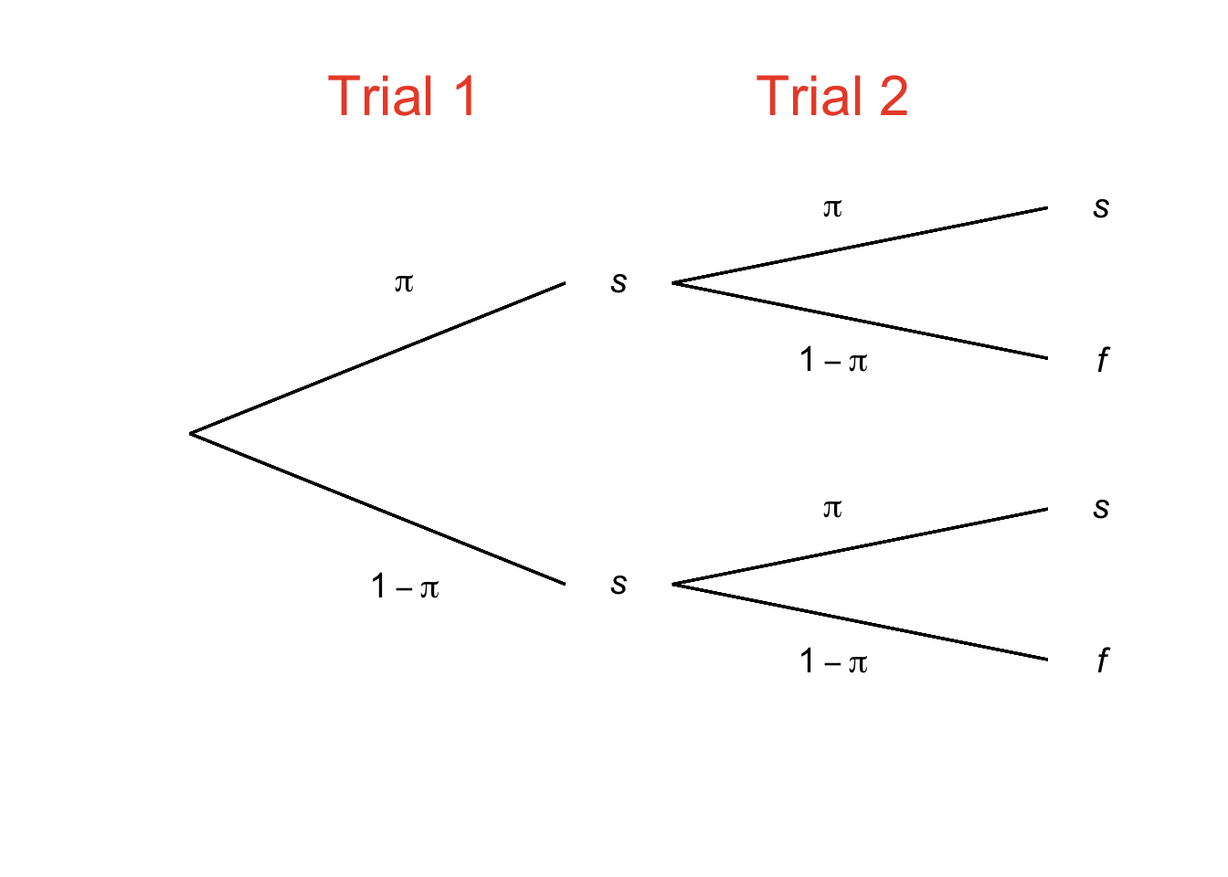
Figure 4.17: Two Binomial Trials

We can use Figure 4.17 to help us see that:

\[p(2s)=\pi^2\] \[p(1s)=(\pi)(1-\pi)+(1-\pi)(\pi)\] \[p(0s)=(1-\pi)^2\]

In general, the likelihood of a set of outcomes is the probability of getting to each outcome times the number of ways to get to that outcome. The probability of each path is known as the kernel probability⁹⁷ and is given by:

\[kernel~probability=\pi^s(1-\pi)^f\]

Given the probability of each path, the overall probability is the sum of the paths. In other words, the binomial likelihood is the product of the kernel probability and the number of possible combinations represented by the kernel probability. The number of possible combinations is given by the combination formula:

\[_NC_s=\frac{N!}{s!f!}\] Put them together, and we have…

4.9.1.1 The Binomial Likelihood Function

\[p(s|N=s+f,\pi)=\frac{N!}{s!f!}\pi^s(1-\pi)^f\] The binomial likelihood function makes it easy to find the likelihood of a set of binomial outcomes knowing only (a) the probability of success on any one trial and (b) the number of trials. For example:

What is the probability of getting exactly 7 heads in 10 flips of a fair coin?

We’ll call heads a success, we know that in the case of a fair coin the probability of heads is 0.5, and $N=10$ trials.

\[p(s=7|\pi=0.5, N=10)=\frac{10!}{7!3!}(0.5)^7(0.5)^3=0.1171875\] 2. What is the probability of drawing three consecutive blue marbles with replacement ⁹⁸ from a jar containing 1 blue marble and 4 orange marbles?

We’ll call blue a success, we know the probability of drawing a blue marble from a jar with one blue marble and four orange marbles is $1/5=0.2$, and $N=3$ trials.

\[p(s=3|\pi=0.2, N=3)=\frac{3!}{3!0!}(0.2)^3(0.8)^0=0.008\] 3. The probability of winning a game of craps at a casino is approximately 49%. If 15 games are played, what is the probability of winning at least 12?

We’ll call winning a success (not much of a stretch there), we are given that $\pi=0.49$, and there are $N=15$ trials. This question specifically asks for the probability of at least 12 successes, which means we are looking for the probability of winning 12 _or 13 or 14 _or 15 games. In other words, we have union probabilities of mutually exclusive events (you can’t win 12 and 13 games out of 15), so we add them.

\[p(s\ge 12|\pi=0.49, N=15)=\frac{15!}{12!3!}(0.49)^{12}(0.51)^3+\frac{15!}{13!2!}(0.49)^{13}(0.51)^2\] \[+\frac{15!}{14!1!}(0.49)^{14}(0.51)^1+\frac{15!}{15!0!}(0.49)^{15}(0.51)^0=0.01450131\]

4.9.1.2 Expected Value and Variance of Binomial Events

A nice property of binomial probability is that the expected value and the variance are especially simple to find. We can still use the typical equation for the expected value:

\[E(x)=\sum_{i=1}^Nx_i p(x_i)\]

but consider that binomial outcomes are binary data and can be assigned values of 1 and 0. For example, let’s consider 2 flips of a fair coin where heads is considered success and is assigned a value of 1. The sample space for s is $\Omega=\{0, 1, 2\}$. As we have noted elsewhere, the probability of 0 heads in 2 flips is 0.25, the probability of 1 heads in 2 flips is 0.5, and the probability of 2 heads in 2 flips is 0.25. Thus, the expected value of s is:

\[E(x)=(0)(0.25)+(1)(0.5)+(2)(0.25)=1\] Thus, in two flips of a fair coin, we can expect one heads. In general, the expected value of a set of $N$ binomial trials with a $p(s)=\pi$ where $s=1$ and $f=0$ is:

\[E(x)=N\pi\] The variance is similarly easy. The variance of a set of $N$ binomial trials with a $p(s)=\pi$ where $s=1$ and $f=0$ is:

\[V(x)=N\pi(1-\pi)\] To illustrate using the general variance formula for the case of two flips of a fair coin (where we have already shown that $E(x)=1$:

\[V(x)=(0-1)^2(0.25)+(1-1)^2(0.5)+(2-1)^2(0.25)=0.25+0.25=0.5\] which is equal to $N\pi(1-\pi)=(2)(0.5)(0.5)$.

4.9.2 Bayes’s Theorem

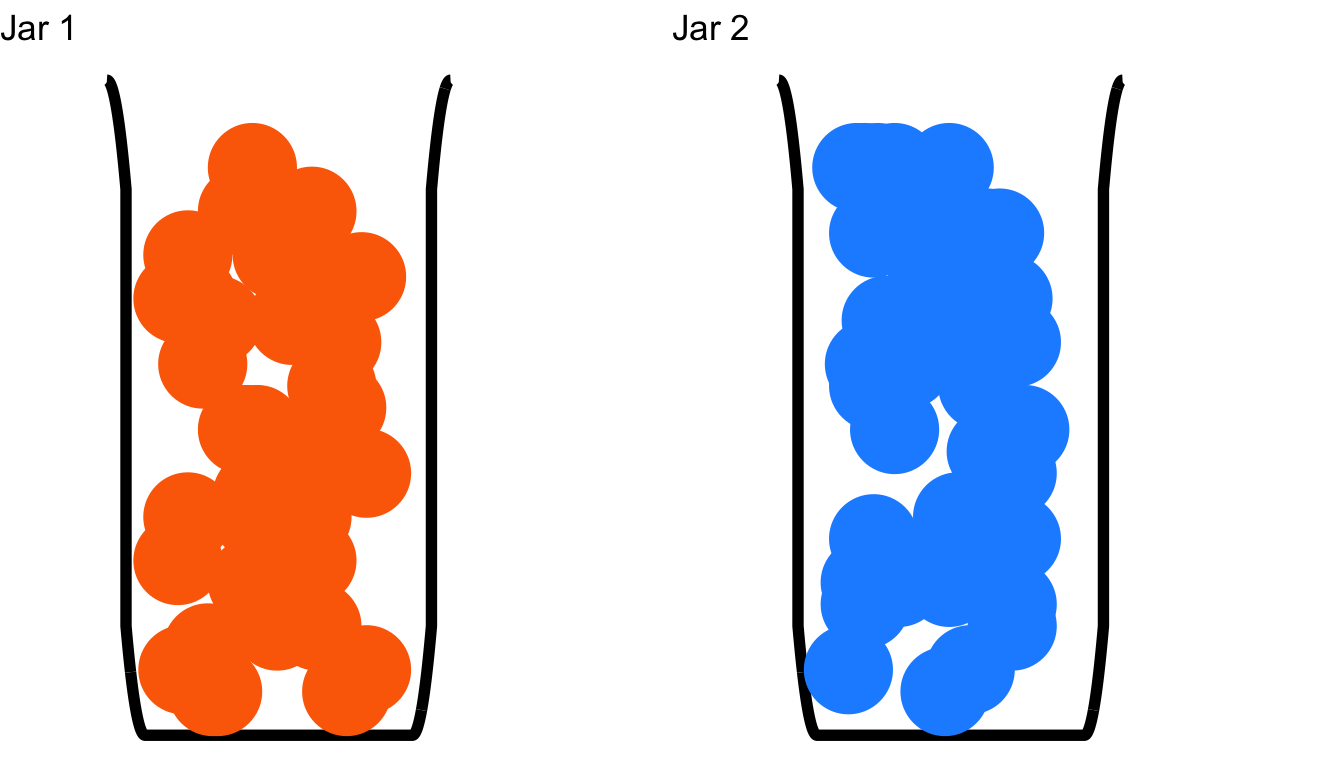
Figure 4.18: The Setup to a Brief Series of Relatively Easy Probability Problems

Please examine the contents of the two poorly-drawn jars in Figure 4.18: Jar 1 is filled exclusively with orange marbles and Jar 2 is filled exclusively with blue marbles. Then, please consider the following questions regarding conditional probabilities:

What is the probability of drawing an orange marble given that you have Jar 1?
What is the probability of drawing a blue marble given that you have Jar 1?
What is the probability of drawing an orange marble given that you have Jar 2?
What is the probability of drawing a blue marble given that you have Jar 2?

If we are drawing from Jar 1, we can only draw orange marbles, so there is a 100% chance of drawing orange given that we have Jar 1 and a 0% chance of drawing blue given that we have Jar 1. The reverse is true for Jar 2: there is a 100% chance of drawing blue and a 0% chance of drawing orange given that we have Jar 2. In this example, the conditional probability of drawing an orange marble or a blue marble depends entirely on what jar we have. In more formal terms, the sample space of the possible events is conditional on what jar we have: if we have Jar 1, then the sample space is $\{Orange,~Orange,~Orange,...\}$; if we have Jar 2, then the sample space is $\{Blue,~Blue,~Blue,...\}$. Yet another fancy way of saying that is to say that the choice of jar reconditions the sample space.

Now let’s add a fifth question about these jars. Imagine that all of the marbles in Jar 1 are still orange and all of the marbles in Jar 2 are still blue, but now the jars are opaque and a marble is drawn without looking inside.

Given that a blue marble is drawn, what is the probability that we have Jar 2?

Since there are no blue marbles in Jar 1 and there are blue marbles (and nothing but) in Jar 2, we must conclude that there is a 100% chance that we have the now-much-less-transparent Jar 2.

Things would be a little trickier if there were a mixture of orange and blue marbles in each jar, or if one jar was somehow more probable to have than the other before drawing, or if there were three, four, or more jars. Fortunately, we have math to help us. Specifically, there is one equation that helps us calculate conditional probabilities, and it’s a pretty important one.

Figure 4.19: Hilariously, this may or may not be a picture of the Reverend Thomas Bayes. Even more hilariously, Thomas Bayes may or may not have been the one who first derived Bayes’s Theorem. The Bayes brand is uncertainty and it is strong

The equation that gives the conditional probability of one event given the other is known as Bayes’s Theorem. Bayes’s theorem follows directly from the definition of conditional probability mentioned abote, that is:

The probability of $A$ and $B$ happening $p(A\cap B)$ is the product of the probability of $A$ given $B$ and the probability of $B$:

\[p(A\cap B)=p(A|B)p(B)\]

Since the designation of the names $A$ and $B$ is arbitrary, we can also rewrite that as:

\[p(A\cap B)=p(B|A)p(A)\]

and since both $p(A|B)$ and $p(B|A)$ are equal to $p(A\cap B)$, it follows that:

\[p(A|B)p(B)=p(B|A)p(A)\]

We can divide both side of that equation by $p(B)$, resulting in:

\[p(A|B)=\frac{p(B|A)p(A)}{p(B)}\]

which is Bayes’s Theorem, although it’s more commonly written with the top two terms of that numerator switched:

\[p(A|B)=\frac{p(A)p(B|A)}{p(B)}\]

Let’s bring back our pair of marble jars to demonstrate Bayes’s Theorem in action. This time, let’s stipulate that there are 40 marbles in each jar. Jar 1 contains 10 orange marbles and 30 blue marbles; Jar 2 contains 30 orange marbles and 10 blue marbles:

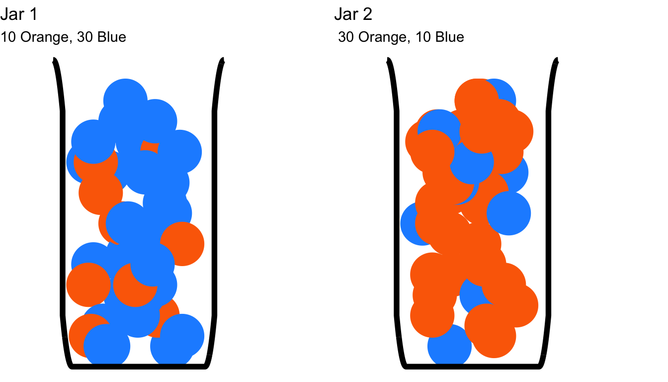
Figure 4.20: The Setup to a Brief Series of Conditional Probability Problems

In this set of examples, let’s assume that one of these jars is chosen at random, but which jar is chosen is unknown. That means that we can reasonably assume that the probability of choosing Jar 1 is the same as the probability of choosing Jar 2. As above, a marble is drawn – without looking inside of the jar – from one of the jars. Here is the first of a new set of questions:

If a blue marble is drawn, what is the probability that the jar that was chosen is Jar 1?

This problem is ideally set up for using Bayes’s Theorem.⁹⁹ The (slightly rephrased) question:

What is the probability of Jar 1 given a blue marble?

is equivalent to asking what $p(A|B)$ is, where event $A$ is choosing Jar 1 and event $B$ is drawing a blue marble. To use Bayes’s Theorem to solve for $p(A|B)$, we are going to need to first find $p(A)$, $p(B|A)$, and $p(B)$.

$\underline{p(A):}$

Event $A$ is Jar 1, so $p(A)$ is the probability of choosing Jar 1. We have stipulated that the probability of choosing Jar 1 is the same as the probability of choosing Jar 2. Because one or the other must be chosen (i.e., the sample space $\Omega=\{Jar~1,~Jar~2\}$ and the probability of choosing Jar 1 or Jar 2 is one (i.e., $p(Jar~1\cup Jar~2)=1$, or equivalently, $\sum\Omega=1$), then:

\[p(A)=\frac{p(A)}{p(A)+p(B)}=\frac{p(A)}{2p(A)}=\frac{1}{2}=0.5\]

$\underline{p(B|A):}$

Event $B$ is (drawing a) blue (marble), so $p(B|A)$ is the probability of blue given Jar 1. If Jar 1 is given, then the sample space for drawing a blue marble is restricted to the probability of drawing a blue marble from Jar 1: Jar 2 and the marbles in it are ignored. Because there are 30 blue marbles and 10 orange marbles in Jar 1 (i.e., $\Omega=\{30~Blue,~ 10~Orange\}$), the probability of $B|A$ – drawing a blue marble given that the jar is Jar 1, is:

\[p(B|A)=\frac{30}{40}=\frac{3}{4}=0.75\]

$\underline{p(B):}$

Again, event $B$ is drawing a blue marble. There is no conditionality to the term $p(B)$: it refers to the overall probability of drawing a blue marble from either jar. Finding $p(B)$ is going to take a bit of math, and we can use a probability tree to help us, too.

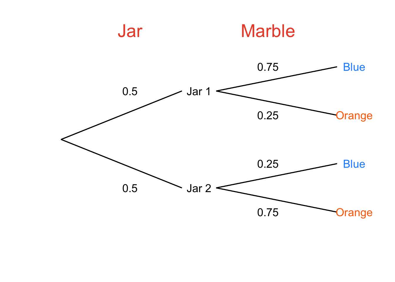
Figure 4.21: Probability Tree for Choosing Jars and Then Drawing Orange and Blue Marbles From Those Jars

There are two ways to get to a blue marble: (1) drawing Jar 1 with 50% probability and then drawing a blue marble with 75% probability, and (2) drawing Jar 2 with 50% probability and then drawing a blue marble with 25% probability. As we do with probability trees, we multiply across to find the intersection probabilities of $Jar~1\cap Blue$ and $Jar~2\cap Blue$ ¹⁰⁰ and add down to find the union probabilities of the two paths that lead to blue marbles to get the overall probability of drawing a blue marble ($p(B)$):

\[p(B)=(0.5)(0.75)+(0.5)(0.25)=0.5\] Now that we know $p(A)$, $p(B|A)$, and $p(B)$, we can calculate $p(A|B)$: the probability that Jar 1 was chosen given that a blue marble was drawn:

\[p(A|B)=\frac{p(A)p(B|A)}{p(B)}=\frac{(0.5)(0.75)}{0.5}=0.75\]

Here’s another question:

What is the probability that Jar 2 was chosen given that a blue marble was drawn?

We can approach this question in two different ways. First, we can use the same steps that we did to solve the first question, with Jar 2 now being event $A$ and drawing a blue marble still being event $B$. Since we know that $p(Jar~1)=p(Jar~2)$, $p(A)$ is still $0.5$. $p(B|A)$ is now the probability of drawing a blue marble from Jar 2, so $p(B|A)$ in this case is equal to $10/40=1/4=0.25$. $p(B)$ is still the overall probability of drawing a blue marble, which remains unchanged: $p(B)=0.5$. Thus, the probability of Jar 2 is:

\[p(A|B)=\frac{p(A)p(B|A)}{p(B)}=\frac{(0.5)(0.25)}{0.5}=0.25\]

The other way we could solve that problem – the much easier way – is to note that if the probability that we have Jar 1 is 0.75, then the probability that we don’t have Jar 1 is:

\[1-p(Jar~1|Blue)=1-0.75=0.25\] I probably could have led with that. Anyway, the probability that we have Jar 1 is 0.75 and the probability that we have Jar 2 is 0.25, meaning that it is three times more probable that we have Jar 1 than that we have Jar 2.¹⁰¹ That lines up with the fact that the proportion of blue marbles is three times greater in Jar 1 than it is in Jar 2.

Now let’s try a slightly trickier question:

After drawing a blue marble from one of the jars, the marble is replaced in the same jar, the jar is shaken, and a second marble is drawn. The second marble drawn is also blue. What is the probability that the jar is Jar 1?

To reduce confusion, let’s add some subscripts to $A$ and $B$: we can add $_1$ to refer to anything that happened on the first draw, and $_2$ to refer to what’s happening on the second draw.

$\underline{p(A_2):}$

Event $A$ is again Jar 1, but this time, $p(A)$ is different. Having already drawn a blue marble from that same jar, we must update the probability that we have Jar 1 based on that new information. In the last problem, we found the probability that we have Jar 1 given that a blue marble was drawn. That probability is our new $p(A)$. Thus, our new $p(A)$ – denoted $p(A_2)$¹⁰² – is $p(A_2|B_1)$: the updated probability of having Jar 1 _in this second draw given that a blue marble was drawn on the first draw:

\[p(A_2)=p(A_2|B_1)=\frac{p(A_1)p(B_1|A_1)}{p(B_1)}=\frac{(0.5)(0.75)}{0.5}=0.75\]

$\underline{p(B_2|A_2):}$

Event $B$ is still (drawing a) blue (marble), and the relative numbers of marbles in Jar 1 is still the same (because we replaced the marble), so $p(B|A)$ is still $30/40=0.75$.

$\underline{p(B_2):}$

The denominator of Bayes’s Theorem, like the $p(A)$ term, also needs to be updated because we no longer believe that having either jar is equally probable. The change happens between the first and second nodes of the probability tree:

Probability Tree for Having a Particular Jar and Then Drawing Orange and Blue Marbles From That Jar Having Once Drawn a Blue Marble From That Jar

Figure 4.22: Probability Tree for Having a Particular Jar and Then Drawing Orange and Blue Marbles From That Jar Having Once Drawn a Blue Marble From That Jar

There are still two ways to get to a blue marble, but the probability associated with each path has changed: (1) drawing Jar 1 with 75% probability and then drawing a blue marble with 75% probability, and (2) drawing Jar 2 with 25% probability and then drawing a blue marble with 25% probability. As before, we multiply across to find the intersection probabilities of $Jar~1\cap Blue$ and $Jar~2\cap Blue$ ¹⁰³ and add down to find the union probabilities of the two paths that lead to blue marbles to get the updated overall probability of drawing a blue marble ($p(B)$):

\[p(B_2)=(0.75)(0.75)+(0.25)(0.25)=0.625\]

With new values for each term of Bayes’s Theorem – $p(A_2)$, $p(B_2|A_2)$, and $p(B_2)$ – we can calculate $p(A_2|B_2)$: the probability that Jar 1 was chosen given that a blue marble was drawn on consecutive draws:

\[p(A_2|B_2)=\frac{p(A_2)p(B_2|A_2)}{p(B_2)}=\frac{(0.75)(0.75)}{0.625}=0.9\] Now we are more certain that we have Jar 1 in light of additional evidence: the probability was 0.75 after drawing one blue marble from the jar, and now that we have drawn two consecutive blue marbles (with replacement) from that jar, the probability is 90%. In other words, drawing two marbles leads to greater confidence that we have the blue-heavy jar in our hands. Additionally, we know that if there is a 90% probability that we have Jar 1, then there is a 1 – 90% = 10% chance that we have Jar 2: it is now nine times more likely that we have Jar 1 than Jar 2. Let’s ask one more question – this one a two-parter – before we move on:

What is the probability that the jar is Jar 1 if the next draw (after replacing the blue marble) is:
1. a blue marble?
2. an orange marble?

I will leave going through all of the steps again as practice for the interested reader and skip to the Bayes’s Theorem results. For part (a), if another blue marble is drawn, then $A_3$ is having Jar 1 given the two previous draws and $B_3$ is drawing a third blue marble:

\[p(A_3|B_3)=\frac{p(A_3)p(B_3|A_3)}{p(B_3)}=\frac{(0.9)(0.75)}{(0.9)(0.75)+(0.1)(0.25)}=\frac{0.675}{0.675+0.025}=0.96\] With three consecutive draws of blue marbles, the probability is high – 96%, to be precise – that we have the majority-blue jar.

Let’s address part (b) of the question: what happens if we draw an orange marble? If we, in fact, were drawing from Jar 1, drawing an orange marble would be far from impossible – there are 10 orange marbles in Jar 1. But, since orange marbles are much more likely to come from Jar 2, having Jar 1 would be less certain than if we had drawn a third consecutive blue marble.

For this part of the question, event $B_3$ is drawing an orange marble on the third draw, and event $A_3$ is having Jar 1 given the information we got from the first two draws. Again, we’ll leave all of the steps as an exercise for the interested reader and skip to the final Bayes’s Theorem equation:

\[p(A_3|B_3)=\frac{(A_3)(B_3|A_3)}{p(B_3)}=\frac{(0.9)(0.25)}{(0.9)(0.25)+(0.1)(0.75)}=0.75\]

…and so the probability that we have Jar 1 takes a step back.¹⁰⁴ Updating is an important feature of conditional probabilities calculated using Bayes’s Theorem. Drawing marbles with replacement from a jar doesn’t change the probabilities associated with those marbles: if the jar contains a lot more orange marbles than blue marbles and we pick three blue marbles in a row, we’d just say “huh, that’s weird” and move on with our lives – low-probability events are not impossible events. But, if we know the relative numbers of marbles in several jars but which jar we have is unknown, then the chances of having one of those jars can constantly be updated as we obtain more information.

If you are still reading this, you may have noticed that I’ve belabored the discussion of jars and marbles to an extent that might suggest that I’m talking about jars and marbles but at the same time I’m not really talking about jars and marbles.

I’m talking about science.

4.9.2.1 Bayes’s Theorem and Statistical Inference

In the labored analogy above, the jars represent hypotheses about the world and the marbles represent data that can support or contradict those hypotheses. A hypothesis can represent a model of how a scientific process works and/or parameters that cannot be directly measured. In the Bayesian framework of evaluating scientific hypotheses, testing different hypotheses is like choosing an opaque, unlabeled jar: there are probabilities associated with each hypothesis being correct (like the probabilities of choosing different jars), we have some idea of the probability of what the data would look like given each hypothesis (like the probability of drawing a kind of marble given the jar), and an idea of the overall probability of the data (like the overall probability of drawing a kind of marble).

When we’re using Bayes’s Theorem to refer to scientific inference, we change the notation in two subtle but important ways: instead of $A$ we use $H$ to mean hypothesis and instead of $B$ we use $D$ to mean data. The resulting equation is:

\[p(H|D)=\frac{p(H)p(D|H)}{p(D)}\]

Each of the terms of Bayes’s Theorem has a special name that reflects its role in the inferential process.

4.9.2.1.1 Terms of Bayes’s Theorem

4.9.2.1.1.1 Prior Probability

$p(H)$, is the probability of the hypothesis; more specifically, it is the prior probability¹⁰⁵ The prior probability (often referred to simply as the prior) is the probability of a given hypothesis before data are collected in a given experiment or investigation. We may initially have no reason to believe that one hypothesis is any more likely than the others under consideration: in that case, prior probabilities can be based on equal assignment.¹⁰⁶ On the other hand, we may have reason to consider some hypotheses as much more likely than others based on our scientific beliefs and/or existing evidence. And, just as we updated $p(A)$ for jars based on marbles, we can use the results of one Bayesian investigation to update $p(H)$ for subsequent investigations – more on that below.

4.9.2.1.1.2 Likelihood

$p(D|H)$ is the probability of the data given the hypothesis, and is known as the likelihood. Any conditional probability is a likelihood – the left side of our Bayes’s Theorem equation ($p(H|D)$) is also a likelihood, but it has its own name so we almost never refer to it as such – hence the name. The likelihood informs us how likely or unlikely the observed data are if a hypothesis is true. The likelihood of the data is typically determined by a likelihood function: if the observed data are close to what the likelihood function associated with a hypothesis would predict, then the likelihood of the data given the hypothesis will be relatively high; if the observed data are way off from the predictions that the likelihood function makes, the likelihood of the data given the hypothesis will be relatively low. How do we know what the likelihood function for a hypothesis should be? Well, sometimes it’s obvious, and sometimes it’s tricky, and sometimes there isn’t one so we use computer simulations to get the likelihood by brute force. In any event, it’s usually not as simple as the marble-and-jar analogy might make it seem, but we will cover that at length in later content.

4.9.2.1.1.3 Base Rate

$p(D)$ is the overall probability of the data and is known as the base rate.^[_Base rate:_The unconditioned probability of observed events.<> In theoretical terms, the base rate – like the probability of drawing a certain type of marble from all jars – is the combined probability of observing the data under all possible hypotheses. In practical terms, the base rate is the value that makes the results of Bayes’s Theorem (as discussed just below, the left-hand side of Bayes’s Theorem is known as the posterior probability) for all of the hypotheses sum to one. That is, if we have $n$ hypotheses, and we have a prior and a likelihood for each of hypotheses $i$, then the base rate is:

\[\sum_{i=1}^n(p(H_i)p(D|H_i)\] Please note that this is precisely the calculation we used for Bayes’s Theorem denominator in the marbles-in-jars problems, just using different terms:

\[~~~p(Jar~1)p(Blue~Marble|Jar~1)\] \[\underline{+~p(Jar~2)p(Blue~Marble|Jar~2)}\] \[\sum_{i=1}^n(p(H_i)p(D|H_i)\]

4.9.2.1.1.4 Posterior Probability

The final term to discuss is the left-hand side of Bayes’s Theorem: the probability of the hypothesis given the data $p(H|D)$, which is known as the posterior probability¹⁰⁷.The posterior probability (often just called the posterior) is the updated probability of a hypothesis after taking into account the prior, the likelihood, and the base rate. In the Bayesian framework of scientific inference, it is the answer we have after conducting an investigation. However, it is not necessarily our final answer: as illustrated in our marbles-in-jars problems, we can update probabilities by obtaining more evidence. In the scientific context, this means that we can use our posterior for one study as the prior for the next study.

4.10 Monte Carlo Methods

I don’t know if you noticed, but the citation date on Kolmogorov’s axioms is 1933. That is, on the scale of mathematical discoveries, incredibly recent! The concept of randomness is not one that humans naturally understand very well (ahem), and it wasn’t until the 20th century that we learned to use randomness to solve problems rather than just to be a problem. Luckily (ha, ha), it was also in the 20th century that we developed the computing power to use repeated random sampling to solve problems that are intractable with analytic methods like calculus.

Monte Carlo methods are named after the Casino de Monte-Carlo (pictured above). One of the developers of the technique had an uncle with a gambling problem who habitually frequented the Monte Carlo Casino.

The practice of using repeated random sampling to solve problems in statistics (and other fields, including physics and biology) is known as using Monte Carlo methods or, equivalently, as using Monte Carlo simulations or Monte Carlo sampling. Here, we will introduce Monte Carlo methods with some relatively straightforward examples.

4.10.1 Random Walk Models

Sticking with the casino theme: let’s imagine a gambler playing craps for $10 per game. On any given game, she has a 49% chance of winning (in which case her total money will increase by $10) and a 51% chance of losing (she will lose $\10)¹⁰⁸. How can we project how her money will be affected by playing the game?

We know that, over the long run, she will win 49% of her games, and we can calculate that the expected value of each gamble is $(\$10)(0.49)+(-\$10)(0.51)= -\$0.20$, meaning that she can expect to lose 20 cents per game. But, gambling doesn’t really work that way: if the gambling experience consisted of periodically handing 20 cents to the casino, nobody would gamble (I think). Our gambler is going to win some games, and she is going to lose some games. It’s possible that she will, over a given stretch, win more games than she loses and will leave the craps table when she hits a certain amount of winnings. It’s also possible that she will lose more games than she wins and will leave the craps table when she is out of money. Or, she might not win as much as she wants nor lose all her money, but get tired after a certain amount of games.

We can model our hypothetical gambler’s monetary journey using a random walk model¹⁰⁹. A random walk model (sometimes more colorfully called the drunkard’s walk) is a (usually visual) representation of a stochastic¹¹⁰ process, and has been applied in psychology to the process of arriving at a decision, in physics to the motion of particles, in finance to the movement of markets, and in other fields.

In the case of our gambler, let’s say she has $100 with her. She will stop playing if:

she wins a total of $100 (and finishes with $200)
she loses the $100 (and finishes with $0)
she plays 200 games and gets tired (honestly this one is just so the graphs fit on the page)

We can see how one simulation based on Monte Carlo sampling plays out in Figure 4.23.

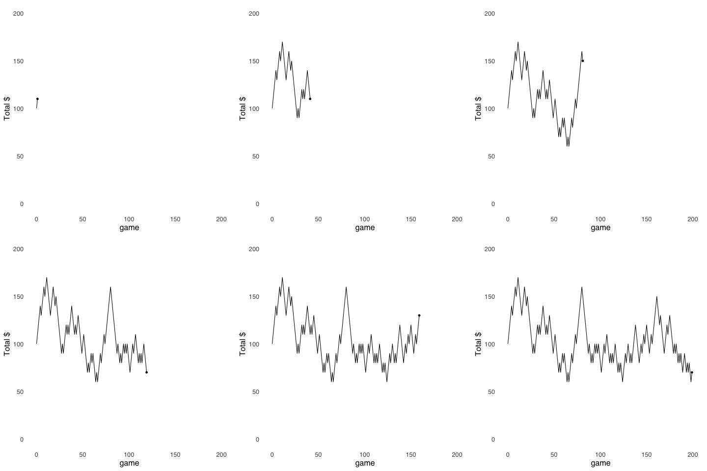
Figure 4.23: A Random Walk

On this specific walk, our gambler starts strong, winning her first four games and nine of her first 11 to go up $70 to a peak of $70. The rest of her session doesn’t go quite so well, but she is still not broke after 200 games: she walks away with $70, presumably to be spent on overpriced adult beverages by the pool.

But, it is important to note that this is just one possible set of circumstances. To get a better idea of what she could expect, we would want to simulate the experience lots of times. The expected value here (still $-\$0.20$) is less interesting a prediction than how many times she leaves having hit her goal earnings, how many times she loses all her money, and how many times she ends up somewhere inbetween. A small set of multiple random walk simulations is visualized in Figure 4.24.

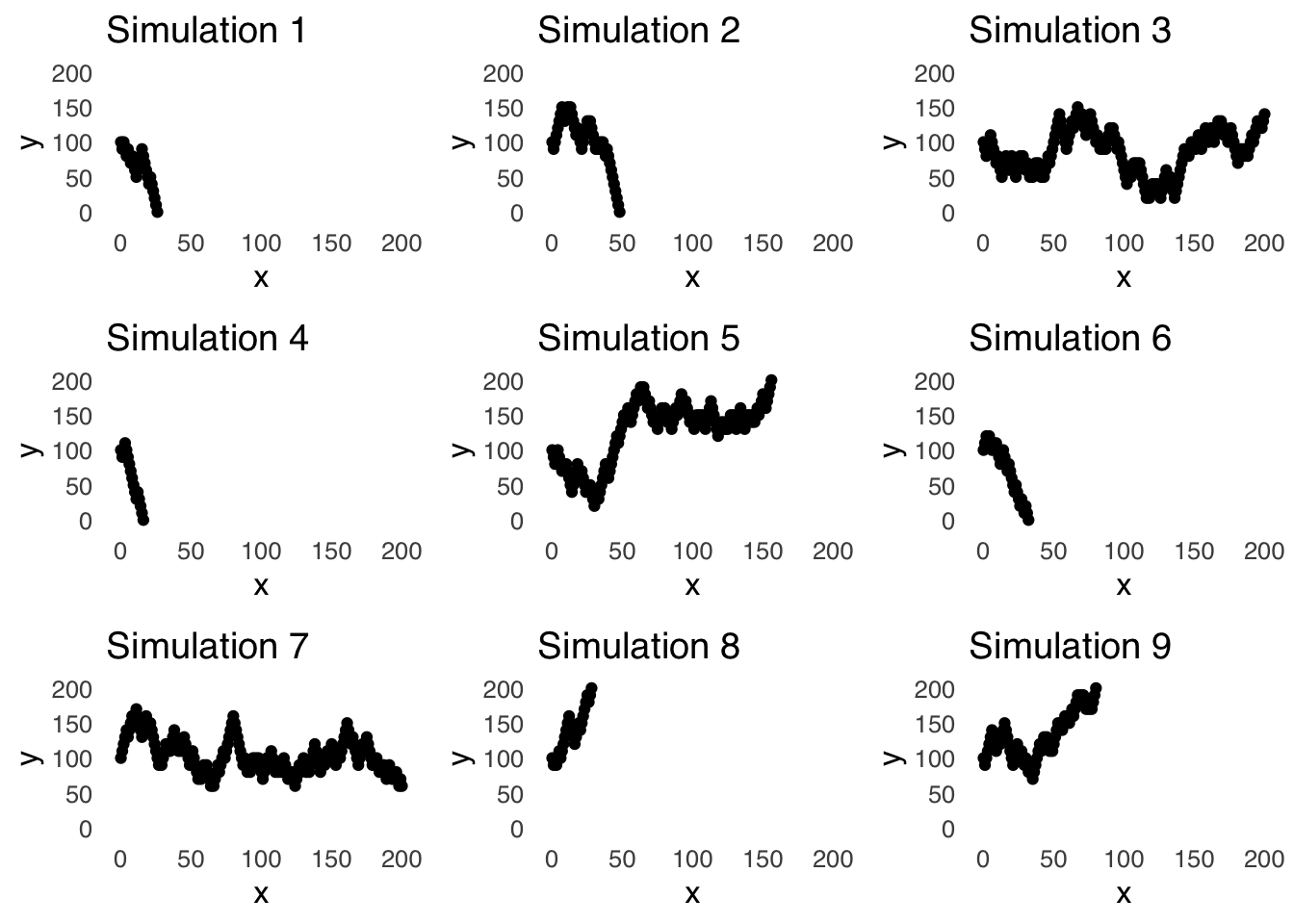
Figure 4.24: 9 Random Walks

In these 9 simulations, our gambler leaves the game up $100 three times, loses her whole bankroll four times, and leaves after 200 games twice.

Typically, simulations are run in greater numbers – just as one run can appear to be lucky or unlucky, a handful of simulations is rarely compelling. Thus, let’s try a greater number of random walks. In a run of 1,000 simulations (don’t worry, we won’t make a figure for this one), in 424 of them (42.4%), our gambler left with $200, in 449 (44.9%) of them, she left with $0, and in 127 (12.7%), she left the table after 200 games having neither hit her goal nor having lost all of her money. Please note how much different this is than what would be predicted using the expected value of each gamble: if she lost $0.20 every time she played (which, of course, is impossible, because she could either win $10 or lose $10), then she would be guaranteed to leave with $60. The simulation results are likely a more meaningful result because it describes likely outcomes based on realistic behavior.

4.10.2 Markov Chain Monte Carlo (MCMC)

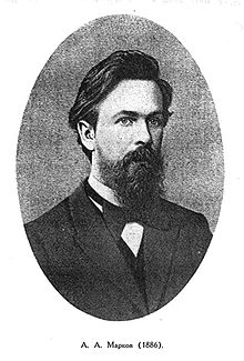
Figure 4.25: Andrey Markov

A Markov Chain, like the random walk model (the random walk model is considered a special case of a Markov chain), is a representation of a stochastic process that moves in steps. In the Markov chain, the steps are known as transitions between different states that occur with some probability. Markov chains have specific applications in psychology and group dynamic, but, more importantly for us, will have important implications for the incorporation of stochastic searches in statistics.

One psychological application of Markov Chain models is in learning and memory. For example, in William Estes’s (1953) 3-state learning model ¹¹¹ there are three possible states for an item to be learned: the item could be in the unlearned state, in a short-term state (where it may be temporarily memorable but not for long), or in a long-term state (that is relatively permanent but from which things can be forgotten).

According to the Estes model (see Figure 4.26), during the course of learning, an item starts out in an unlearned state – which we will call $1$ – and will stay in state $1$ with probability $a$. Given that it is assumed that the item stays state $1$ with probability $a$, it follows that it will leave that state with probability $1-a$. If the item leaves the unlearned state, it has two places to go: the short-term state – state $2$ – and the long-term state – state $3$. We can designate the probability of going to state $2$ as $b$ and the probability of going to state $3$ as $1-b$: therefore the probability of an item leaving state $1$ and going to state $2$ as $(1-a)(b)$ and the probability of an item leaving state $1$ and going to state $3$ as $(1-a)(1-b)$. We can then continue, designating the probability of an item in state $2$ and staying there as $c$ and of an item leaving state $2$ as $1-c$, etc., etc., as shown in Figure 4.26.

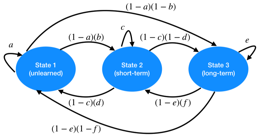
Figure 4.26: A Three-State Markov Chain Model

Just as we designated the probabilities of winning and losing in the random walk, we can designate the probabilities $a$, $b$, $c$, $d$, $e$, and $f$ and use those probabilities to repeatedly simulate the stochastic motion of items between memory states using the Markov Chain model.

Far more important for us, though, is that we can use Markov Chain Monte Carlo methods to generate probability distributions about scientific hypotheses by moving numeric estimates from beginning states to increasingly more probable states. We’ll talk about that later.

4.11 Summary Information

4.11.1 Glossary

Event (or Outcome - we will use them interchangeably): A thing that happens. Roll two dice and they come up 7 –- that’s an event (or, an outcome). Flip a coin and it comes up heads – that’s an outcome (or, an event)

$p(A)$: the probability of event A. For example, if event A is the probability of a coin landing heads, we can write: \[p(A)=0.5\] or we can spell out heads instead of using A: \[p(heads)=0.5\] $\neg$ A: a symbol for not A, as in “event A does not happen.” If event A is a coin landing heads, we can say \[p(\neg~A)=0.5=p(tails)\]

Trial: A single occurrence where an event can happen. “One flip of a coin” is an example of a trial.

Defined experiment: An occurrence or set of occurrences where events happen with some probability. “One flip of a coin” is a defined experiment. “Three rolls of a single sided die” is a defined experiment. “On Tuesday” is a defined experiment if you’re asking, “what’s the probability that it will rain on Tuesday.” Please note that a defined experiment could be one trial or it could comprise multiple trials.

Sample space (symbolized by $\Omega$ or $S$): All possible outcomes of a defined experiment. For example, if our defined experiment is “one flip of a coin,” then the sample space is one heads and one tails, which we would symbolize as: $\omega={H,T}$

Elementary event: An event that can only happen one way. If we ask, “what is the probability that a coin lands heads twice in two flips, there’s only one way that can happen: the first flip must land heads and the second flip must also land heads.

Composite (or compound) event: An event that can happen multiple ways. If we ask, “what is the probability that a coin lands heads twice in three flips, there are three ways that can happen: the flips go heads, heads, tails, the flips go heads, tails, heads, or the flips go tails, heads, heads.

Mutual exclusivity: A condition by which two (or more) events cannot both (or all) occur. In one flip of a coin, heads and tails are mutually exclusive events.

Collective exhaustivity: A condition by which at least one of a set of events must occur in a defined experiment. For one flip of a coin, heads and tails are said to be collectively exhaustive events because one of them must happen.

Independent events: Events where the probability of one event does not affect the probability of another. For example, the probability that your birthday is July 20 is totally unaffected by the probability that a randomly chosen person that is unrelated to you is also July 20.

Dependent events: Events where the probability of one event does affect the probability of another. The probability of a twin having a birthday on July 20 is very closely related to the probability of her twin sister having a birthday on July 20.

Union (symbolized by $\cup$): or. As in, “what is the probability that it will rain on Tuesday or Friday of next week?” We may rephrase that question as “what is the union probability of rain on Tuesday or Friday?”

Intersection (symbolized by $\cap$): and. As in, “what is the probability that it will rain on Tuesday and Friday of next week?” or “what is the intersection probability of rain on Tuesday and Friday?” Intersection probability is also referred to as conjoint or conjunction probability.

4.11.2 Formulas

4.11.2.1 Intersections and Unions

Probability of A and B:

If $A$ and $B$ are independent, then $p(B|A)=p(B)$

\[p(A\cap B)=p(A)p(B|A)\] Probability of A and B and C:

\[p(A\cup B \cup C)=p(A)p(B|A)p(C|A\cap B)\]

Probability of A or B or C (if A and B are mutually exclusive):

Note: if any pair of events are mutually exclusive, then the probability of any interaction involving them is 0. For example, given events $A$, $B$, and $C$, if $A$ and $B$ are mutually exclusive, then $p(A\cap B)=0$ and $p(A\cap B \cap C)=0$

\[p(A\cup B)=p(A)+p(B)-p(A\cap B)\]

4.11.2.2 Permutations and Combinations

$n$ things permuted $r$ at a time:

\[_nP_r=\frac{n!}{(n-r)!}\] $n$ things combined $r$ at a time:

$_nC_r$ can also be written: \[_{s+f}C_s=\frac{(s+f)!}{s!f!}\] which will be helpful in the context of the Binomial Likelihood Function

\[_nC_r=\frac{n!}{r!(n-r!)}\]

4.11.2.3 Binomial Probability

The Binomial Likelihood Function (the probability of $s$ successes and $f$ failures in $N=s+f$ trials):

\[p(s|N=s+f, ~\pi)=\frac{N!}{s!f!}\pi^s(1-\pi)^f\]

4.11.2.4 Conditional Probability

Bayes’s Theorem:

also known as \[p(H|D)=\frac{p(H)p(D|H)}{p(D)}\] where $H$ is a scientific hypothesis and $D$ is the observed data

\[p(A|B)=\frac{p(A)p(B|A)}{p(B)}\]

4.12 Bonus Content

4.12.1 Why is the factorial of zero equal to one?

Algebraic answer:

The factorial of any number is that number multiplied by the factorial of that number minus one:

\[4!=4\times 3\times 2 \times 1= 4 \times 3!\] \[3!=3\times 2\times 1=3 \times 2!\] \[2!=2\times 1=2 \times 1!\] \[n!=n(n-1)!\]

Thus:

\[1!=1\times 0!\]

throw in some simple division:

\[\frac{1!}{1}=\frac{1\times 0!}{1}\] and thus:

\[1=0!\]

Calculus answer

The factorial function $n!$ is generalized to the gamma function $\Gamma (n+1)$. R software has both a built-in factorial function and a built-in gamma function: you can use both to see the relationship, for example:

gamma(6)

## [1] 120

factorial(5)

## [1] 120

gamma(1)

## [1] 1

factorial(0)

## [1] 1

The gamma function of $n+1$, is defined as:

\[\Gamma (n+1)=\int_0^{\infty}t^{n}e^{-t}~dt.\] Plugging in $n=0$, $t^0=1$, and thus:

\[\Gamma (1)=\int_0^{\infty}e^{-t}~dt=e^{-t}=\left[-e^{-t}\right]_0^\infty=-e^{-\infty}+e^0=0+1=1\]

4.12.2 Excerpts from Statistics for Everybody by D. Barch, reprinted with permission from the author

4.12.2.1 The Law of Large Numbers and the Gambler’s Fallacy

The tendency to believe that event A is less likely to occur after a long run of event A occurring is known as the Gambler’s Fallacy. That fallacy (a fallacy is an illogical line of reasoning) takes its name from the tendency of gamblers to think that after a long string of losses that they are due for a win. Well, they are due for wins – if they continue to play the game forever (and have the means to do so) – but not on any one given trial. So, after ten consecutive heads, would you put a lot of money on tails? You should not change your betting behavior in any way (if anything, shouldn’t you suspect that the coin is messed up and bet on heads?).

4.12.2.2 The Linda Problem and the Conjunction Fallacy

In the early 1980s, Cognitive Psychologist Daniel Kahneman, working with his longtime collaborator Amos Tversky, handed a flyer to 88 undergraduates at the University of British Columbia (UBC). In that flyer read the following description of a fictional woman named Linda:

“Linda is 31 years old, single, outspoken, and very bright. She majored in philosophy. As a student, she was very concerned with issues of discrimination and social justice, and also participated in anti-nuclear demonstrations.” (Tversky & Kahneman, 1983)

Below that passage was a list of 10 statements about Linda, including “Linda is a teacher in an elementary school,” and “Linda works in a bookstore and takes Yoga classes,” and the students were asked to rank-order the probability of each of the statements. Tversky and Kahneman were really only interested in responses these three of the 10 statements:

Figure 4.27: A Linda. Not necessarily THE Linda, though.

Linda is a bank teller
Linda is active in the feminist movement
Linda is a bank teller and is active in the feminist movement.

As Tversky and Kahneman had hypothesized, the majority (85%) of students ranked “active in the feminist movement” above “bank teller and is active in the feminist movement” and, most importantly, ranked both above “bank teller.” The researchers pointed out that such a ranking was impossible according to the rules of intersection probability. Let’s let “active in the feminist movement” be event A and “bank teller” be event B. The intersection (or conjunction, as noted above in the definition for intersection probability) probability of events A and B is:

\[p(A\cap B)=p(A)p(B)\].

Since probabilities are values between 0 and 1, there are no two probabilities that you can multiply together to get a number greater than any one of those probabilities. Thus, it is always the case that:

\[p(A\cap B)\le p(B)~where~p(B) < p(A)\].

With the only ways that $p(A\cap B)$ can be equal to either $p(A)$ or $p(B)$ is if the probability of one or both of the events is equal to 1. This is known as the conjunction rule.

Tversky and Kahneman pointed out that by ranking the probability that Linda was a feminist bank teller higher than the probability that Linda was simply a bank teller, the UBC undergraduates were violating the conjunction rule and committing the conjunction fallacy: assessing the probability of the conjunction as greater than the probability of one of the events. This, they argued, was irrational based on the rules of probability theory, and showed that people were making judgments based on heuristics – quick rules of thumb that we may rely on in place of analytic reasoning. Linda, Tversky and Kahneman argued, was so representative of a person that would be active in the feminist movement that participants in the experiment thought, “well, she doesn’t seem like the bank teller type, but if she is, surely she is active in the feminist movement in her spare time and is not just a bank teller.”

Since the seminal paper from Tversky and Kahneman, other research has been conducted to explain why people commit the conjunction fallacy. The principal antagonist to the Tversky and Kahneman viewpoint has been Gerd Gigerenzer, who has argued (Gigerenzer, 1996; Hertwig & Gigerenzer) that those same heuristics help us make quick and relatively smart decisions about the world around us. Still, for our purposes, let’s keep in mind that, statistically speaking, the conjunction rule should not be violated.

Event (or Outcome - we will use them interchangeably): A thing that happens. Roll two dice and they come up 7 –- that’s an event (or, an outcome). Flip a coin and it comes up heads – that’s an outcome (or, an event)↩︎
Sample space (symbolized by $\Omega$ or $S$): All possible outcomes of a defined experiment. For example, if our defined experiment is “one flip of a coin,” then the sample space is one heads and one tails, which we would symbolize as: $\omega={H,T}$↩︎
Mutual Exclusivity: A condition by which two (or more) events cannot both (or all) occur. In one flip of a coin, heads and tails are mutually exclusive events.↩︎
Intersection ($\cap$): the co-occurence of events; the intersection probability of event $A$ and event $B$ is the probability of $A$ and $B$ occurring.↩︎
Probability Symbols: $p(x)$: the probability of $x$. $\cap$ (cap): and; intersection. $\cup$ (cup): or, union. $\neg$: not. $|$: given↩︎
Conditional Probability: a probability that depends on an event, a set of events, or any other restriction of the sample space↩︎
Defined experiment: An occurrence or set of occurrences where events happen with some probability.↩︎
Please note that there are several ways to express probabilities – as fractions, as proportions, or as percentages – and all are equally fine.↩︎
Trial: A single occurrence where an event can happen.↩︎
Sampling with replacement: The observation of events that do not change the sample space↩︎
Independent Events: Events where the probability of one event does not affect the probability of another.↩︎
The concepts of sampling with replacement and independent events are closely related: we can define sampling with replacement as sampling in such a way that each sample is independent of the last.↩︎
Sampling without Replacement: The observation of events that change the sample space↩︎
Dependent Events: Events where the probability of one event affects the probability of another.↩︎
Sampling without replacement and dependent events are related in the same way that sampling with replacement and independent events are: sampling without replacement implies dependence between events.↩︎
note that we cannot use the simplification $p(B|A)=p(B)$ because these are not independent events↩︎
In general, the intersection probability of independent events is the product of their individual probabilities: \[for~independent~A,~B,~C:\] \[p(A\cap B\cap C ... )=p(A)p(B)p(C)...\]↩︎
There are going to be several gambling-related examples in our discussion of probability theory, and I really don’t mean to encourage gambling. But much of our understanding of probability theory comes from people trying to figure out how games of chance work (that and insurance). When we consider how much of the rest of the field of statistics was derived to justify and promote bigotry, though, promoting gambling isn’t bad by comparison. ↩︎
One can win smaller amounts of money for picking all four digits in any order, or for picking the first three digits in the correct order, or for picking the last three digits in the correct order…it gets complicated. I know all this because my maternal grandparents loved The Numbers Game (almost as much as they hated each other) and their strategies were frequent topic of conversation whenever I was at their house. Anyway, for simplicity’s sake, let’s just focus on the jackpot.↩︎
We know from studying probability theory that outcomes that seem more random are not more random at all: “3984” and “7777” are precisely as likely as each other to happen. So why do numbers like “7777” or “1234” stand out? It’s the cognitive illusion caused by salience: there are just a lot more number combinations that don’t look cool than number combinations that do, and the cool ones stick out while all the uncool ones don’t get remembered.↩︎
“A well-shuffled deck of ordinary playing cards” is a term that teachers are legally required (I think – don’t google that) to use when teaching probability theory – it just means that each card in the deck has an equal ($1/52$) chance of being dealt.↩︎
The value of card combinations in games like poker mostly track with the probabilities of those combinations – for example, a pair of aces is more likely and also less valuable than three aces – and sometimes are based on arbitrary rules to improve game play – for example, a pair of aces is more valuable but just as probable to get as a pair of kings, but having relative ranks of cards limits ties and improves gameplay.↩︎
Union ($\cup$): the total sum of the occurrence of events; the union probability of event $A$ and event $B$ is the probability of $A$ or $B$ occurring.↩︎
The days and times that people are born are not really random but let’s temporarily assume they are for the sake of this example.↩︎
The union probability of three mutually exclusive events $p(A)+p(B)+p(C)$ uses the exact same equation, it’s just that all of the intersection terms are 0.↩︎
As the most likely outcome, 7, in addition to being the expected value, is also the mode. And, since there are precisely as many outcomes less than 7 as greater than 7, it’s also the median.↩︎
Only one of the three elements is named after an actual tree part, a fact that I never thought about before now but it kind of bums me out.↩︎
for more on similar cognitive illusions regarding probability, see the bonus content below↩︎
Elementary Events: events that can only happen in a single way.↩︎
Composite (or Compound) Events: events that can be broken down into multiple outcomes; collections of elementary events (note: in this context composite and compound are identical and will be used interchangeably).↩︎
That is not to say that the probabilities of all elementary events in a sample space are always equal to each other – for example, the probability of the elementary events me winning gold in men’s figure skating at the next Winter Olympics and an actually good skater winning gold in men’s figure skating at the next Winter Olympics are most certainly not the same – but in this case, they are.↩︎
This is a good time to point out that $0!=1$. You can live a long, healthy, and scientifically fruitful life just taking my word for it on that, but for two (hopefully compelling) explanations please see the bonus content down below.↩︎
Permutation: a combination with a specified order↩︎
Combinations: arrangements of items in no specified order_↩︎
This was, verbatim, a question that I got right for my team at pub trivia mainly because I had just taught a lecture on probability theory and the combination formula was fresh in my head. Also, unless a trip is going to be like years long, anything more than one book is too ambitious for me↩︎
Odds: Relative probability ↩︎
Likelihood: a conditional probability↩︎
In common conversation, the terms probability, likelihood, and odds are used interchangeably and without too much confusion. In statistics, the distinctions between the terms are meaningful: probability can refer to any probability, while likelihood refers specifically to a conditional probability and odds refers specifically to a relative probability.↩︎
Binomial Trial: a defined experiment with two possible outcomes; also known as a Bernoulli trial↩︎
Kernel Probability: The probability of an elementary outcome↩︎
Binomial trials are always based on the assumption of sampling with replacement.↩︎
The term inverse probability has been used – mostly in the past and originally derisively – for the kinds of broader probability problems to which this problem is an analogy. If what is the probability that marble x is drawn from jar y is a probability problem, then what is the probability that the jar is jar y given that marble x was drawn from it is the inverse of that. But, today, such problems are more appropriately referred to as Bayesian probability problems.↩︎
We could also find the intersection probabilities of $Jar~1\cap Orange$ and $Jar~2\cap Orange$, but those aren’t really that important for this problem right now.↩︎
Another way of saying the probability is three times greater is the odds in favor of having Jar 1 are 3:1, and another way of saying that is the odds ratio for having Jar 1 is 3. But, we’ll get to that in the section on odds.↩︎
We could also go without the subscripts and just write \[p(A)=0.75,\] keeping in mind the $p(A)$ has been updated. Mathematical notation is supposed to clarify problems rather than to make them more difficult, so whichever approach is more understandable for you is best.↩︎
We still don’t really care about $p(Orange)$.↩︎
For this particular example, that step goes back precisely to where the probability was after the first draw of a single blue marble, but that’s not necessarily the case: the probability will go down, but not necessarily by the same amount that it went up before – that just happened because of the symmetry of 0.75 and 0.25 around 0.5.↩︎
Prior Probability: The probability of a hypothesis before being conditioned on a specified set of evidence.↩︎
Equal-assignment-based prior probabilities are fairly common and are known as flat priors↩︎
Posterior Probability: The probability of a hypothesis conditioned on a set of evidence.↩︎
Dear gambling aficonados: for the purposes of this example, we’ll ignore all the side bets and all that.↩︎
Random walk model: a representation of a series of probabilistic shifts between states.↩︎
Stochastic: Random or describing a process that involves randomness↩︎
this is a not an endorsement of this model on my part↩︎


If	\(A\)	is in the first position, then	\(B \cup C \cup D \cup E\)	can be in the second position
	\(B\)		\(A \cup C \cup D \cup E\)
	\(C\)		\(A \cup B \cup D \cup E\)
	\(D\)		\(A \cup B \cup C \cup E\)
	\(E\)		\(A \cup B \cup C \cup D\)