Chapter 13 Factorial Analysis
13.1 Factorial Between-Groups ANOVA
The one-way between-groups ANOVA design handles situations where there is one independent variable – also known as a factor – that has three or more levels (when there is one factor that has one or two levels, we use \(t\)-tests). Often, we are interested in the effects of more than one independent variable factor at a time.
For example, let’s imagine the case where a social psychologist is interested in how the independent variables mood and social situation – and the combination of mood and social situation impact stress levels. To manipulate the mood factor, participants are randomly assigned to watch one of three brief video clips that have been shown (and validated) to induce positive, neutral, or negative moods, respectively.


Figure 13.1: Pictured L-R: Selected Participants in the Positive, Neutral, and Negative Induced-Mood Conditions
To manipulate the social situation factor, participants are randomly assigned to one of two conditions: a setting populated with actors who are trained to behave in a supportive manner, or a setting populated with actors trained to act antagonistically.


Figure 13.2: Pictured L-R: Selected Participants in the Supportive and in the Antagonistic Social-Situation Conditions
Participants are each shown one (and only one) of the mood-inducing videos and then brought to a room with actors performing either the supportive or the antagonistic roles (and not both); the participants interact with the actors for 15 minutes. The dependent variable for this experience – stress – is measured by levels of cortisol in saliva samples taken following the social interaction.
In this example, mood and social situation are between-groups factors: as noted, each participant sees one and only one of the three videos and interacts with one and only one of the two lab-manufactured situations (if participants saw all the videos, then mood would be a within-groups factor; similarly, if participants experiences both social situations, then social situation would be a within-groups factor). That means that there are six possible combinations of the factors – \(3\) levels of the stress variable times \(2\) levels of the social situation variable (see Table ??), and therefore this experiment requires six totally different groups of participants in each combination of the two factors in order to be a totally between-groups factorial experiment, and every participant experiences one and only one combination of the two factors. Let’s say that there are \(n=30\) hypothetical participants in each combination of hypothetical experimental conditions. Because there are \(3\) levels of the mood variable and \(2\) levels of the social situation variable, there would be \(3 \times 2 \times 30 = 180\) total hypothetical people who participate, but we still refer to the design as having \(n=30\) for both mathematical purposes (the \(n\) in the calculations refers to the per-group number of participants) and for reporting purposes (if another researcher, for example, were to read our research and wanted to modify our hypothetical experiment to add or subtract variables or variable levels, the number of participants per group is more relevant than the total number of participants that we had).
| Mood | |||
|---|---|---|---|---|
Positive | Neutral | Negative | ||
Situation | Supportive | Positive Mood | Neutral Mood | Negative Mood |
Antagonistic | Positive Mood | Neutral Mood | Negative Mood | |
Any time there are multiple factors – even when one or more of the factors has only two levels – we use factorial ANOVA. and t is a special case of ANOVA anyway.
In these cases, we use a Factorial ANOVA
13.1.0.1 Main Effects and Interactions
Main effects are the observed effects of each factor by themselves. Interactions are effects present when multiple treatments are given that are different than the effects present for those treatments applied by themselves.
An effect is called a main effect only if it is significant (otherwise, there is no observed effect). In the example above, a main effect of mood would indicate that the mood factor causes significant changes in the dependent variable; a main effect of situation would indicate that the situation factor causes significant changes in the dependent variable. As with main effects, an interaction is technically only really an interaction if it is statistically significant (but that rule is a lot softer because we don’t have great ways to talk about non-significant factor combinations). Interactions indicate that different combinations of the two factors cause variance in the dependent variable that is independent of the influence of the two factors by themselves.
In an ANOVA analysis, by the strict definition of ANOVA that holds that the \(n\) is the same in all groups, factors and interactions are each sources of unique variance in the dependent variable; that is to say, they are orthogonal.
When \(n\) is not uniform across groups, then factors and interactions are not orthogonal and therefore do not contribute unique variance in the dependent variable: the variance associated with different sources overlaps. Those are cases in which we use general linear models (GLMs) to analyze the data, and different types of estimates for the sums of squares (types I, II, & III).
But that is a concern for another chapter
The key reason to use factorial ANOVA is that we are interested in interactions. It is perfectly good and natural for a scientist to be interested in more than one thing at the same time, and sometimes those things might be measurable by the same quantity. For example: a neuroscientist studying the amygdala might be interested in how different stimuli, time of day, personal experiences, ambient temperature, age, gender identification, and all kinds of other factors influence amygdala activation. It might be tempting to test different factors in the same experiment, but researchers shouldn’t do so unless they are interested in how those factors interact with each other. That doesn’t mean that a factorial experiment is ill-advised if it does not result in a significant interaction – that, of course, is why we try things in science – but only that there needs to be interest in examining if there is an interaction to justify the design. The reason for that is factorial designs require substantial resources to run. In a factorial design, one needs equal numbers of observations for each combination of factors. Thus, the amount of factors either multiplies the number of participants you need (for between-subjects factors) or divides the number of observations in each condition per participant (for within-subjects factors). For example, a two-way independent-groups design with \(3\) factor levels for each factor requires \(9\) total groups to cover each of the \(3\times3\) combinations; if the interaction is not of interest, two experiments using one-way independent groups designs would require just \(6\) groups of participants. In addition to efficiency, interpreting and explaining interactions is complex enough when the interaction is meaningful; attempting to explain an observed interaction for things for which an interaction is irrelevant would be considerably more difficult.
13.1.0.2 Illustrating Main Effects and Interactions Using Our Example
As noted for the example described above, \(n = 30\), and there are \(3 \times 2 = 6\) total combinations of levels of our independent variables. Please keep this in mind: there are going to be \(6 \times 30 = 180\) observations, and those \(180\) numbers are going to have a certain amount of variance, and no method of analyzing that variance will ever create more variance.
13.1.0.2.0.1 No main effects or interaction
Since this is a completely made-up example, there’s no harm in completely making up some data to go with it. First, let’s suppose that mood and social situations both have no impact whatsoever on people’s stress levels. In this (made-up and not at all true!) scenario, stress levels in the population would, on average, be exactly the same in for people in all different moods and in all social situations, and so we would expect that observed stress levels would be about the same on average in every one of our groups. The only thing more absurd than the idea that social situations and moods are meaningless is the idea that we could observe the exact same summary statistics across \(6\) different experimental conditions with continuous data, but that’s exactly the kind of nonsense that is presented in Table ??.
| Mood |
| |||
|---|---|---|---|---|---|
Positive | Neutral | Negative | Situation Means | ||
Situation | Supportive | 500 (25) | 500 (25) | 500 (25) | 500 |
Antagonistic | 500 (25) | 500 (25) | 500 (25) | 500 | |
Mood means | 500 | 500 | 500 | ||
note: fake blood cortisol levels are presented as mean (sd); units are nmol/liter | |||||
That situation illustrates what is basically the null hypothesis: nothing we do does anything. The only variance we would find anywhere in the results is the small – and in this example, identical – variance within each group. There is no variance whatsoever contributed by differences between each group because all \(6\) group means are exactly the same. I can’t stress enough how much observing data with this kind of uniformity will never happen in reality.
13.1.0.2.0.2 One main effect, no interaction
Now, let’s tweak the example data to represent what might happen if there were a true effect of mood but there still wasn’t an effect of social situation; those fake data are in Table ??.
| Mood | ||||
|---|---|---|---|---|---|
Positive | Neutral | Negative | Situation Means | ||
Situation | Supportive | 300 (25) | 500 (25) | 700 (25) | 500 |
Antagonistic | 300 (25) | 500 (25) | 700 (25) | 500 | |
Mood means | 300 | 500 | 700 | ||
note: fake blood cortisol levels are presented as mean (sd); units are nmol/liter | |||||
In this case, positive mood is associated with the lowest stress levels, negative mood is associated with the highest stress levels, and neutral mood is in the middle. The marginal means for the situation variable – the overall averages for situation on the right side of the table, are identical to each other. So, for this set of fake data, mood does something; situation does nothing.
Notice also that we see the same differences in the mood values for each level of the situation variable (i.e., the two inner rows are identical). That means that the means for mood don’t vary between different levels of the situation variable – which also means that the means of the situation variable don’t vary between different levels of the mood variable. All of that implies that in this example, situation and mood do not affect each other.
This is a case where we have a main effect of situation, no effect of mood, and no interaction between the two.
We can also devise a scenario where there is a main effect of mood, but not of situation, and where there is no interaction between the two. That would look like the ersatz data in Table ??.
| Mood | ||||
|---|---|---|---|---|---|
Positive | Neutral | Negative | Situation Means | ||
Situation | Supportive | 300 (25) | 300 (25) | 300 (25) | 300 |
Antagonistic | 700 (25) | 700 (25) | 700 (25) | 700 | |
Mood means | 500 | 500 | 500 | ||
note: fake blood cortisol levels are presented as mean (sd); units are nmol/liter | |||||
Now, note that the values differ between levels of situation, but are identical across the levels of mood, both in the inner rows and on the margins of the table.
13.1.0.2.0.3 Two main effects, no interaction
It’s a little more realistic to posit that there would be effects of both mood and situation on stress levels (although the data here are still very much fake). One such scenario is presented in Table ??.
| Mood | ||||
|---|---|---|---|---|---|
Positive | Neutral | Negative | Situation Means | ||
Situation | Supportive | 300 (25) | 400 (25) | 500 (25) | 400 |
Antagonistic | 500 (25) | 600 (25) | 700 (25) | 600 | |
Mood means | 400 | 500 | 600 | ||
note: fake blood cortisol levels are presented as mean (sd); units are nmol/liter | |||||
In Table ??, the marginal means are different across levels of mood and across levels of situation: blood cortisol measurements for participants in the positive mood condition are lower than the measurements for participants in the neutral mood condition which are lower than the measurements for participants in the negative mood situation; measurements for participants in the supportive situation condition are lower than those for participants in the antagonistic situation condition. But the patterns of the means are similar across combinations of the two. The mean levels increase by the same amount across different levels of mood in each of the situation row. (between each cell from left to right, the means go up by 100 nmol/liter). The mean levels also increase by the same amount across different levels of situation in each of the mood columns (between each cell, the means go up top to bottom by 200 nmol/liter).
Thus, both of the factors mood and situation affect stress independently; the changes are consistent across levels of each factor regardless of the level of the other factors. This, then, is an example of observing two main effects but no interaction.
13.1.0.2.0.4 Interaction, no main effects
The three examples we’ve examined so far all represent scenarios where the two factors do not interact. The following three represent scenarios where there is an interaction; and we’ll start with a (bizarre, even for this set of examples) situation where there is only an interaction and no main effects. Those absurd and, as always, super-fake data are presented in Table ??
| Mood | ||||
|---|---|---|---|---|---|
Positive | Neutral | Negative | Situation Means | ||
Situation | Supportive | 300 (25) | 500 (25) | 700 (25) | 500 |
Antagonistic | 700 (25) | 500 (25) | 300 (25) | 500 | |
Mood means | 500 | 500 | 500 | ||
note: fake blood cortisol levels are presented as mean (sd); units are nmol/liter | |||||
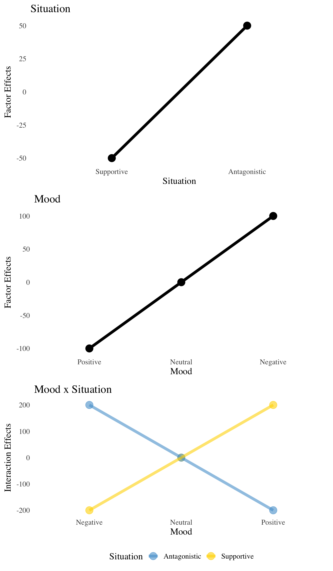
The marginal means indicate absolutely nothing: they’re all the same! If we were only to look at the marginal means, we might conclude that neither mood nor situation has any effect whatsoever. However, the interaction means on the inside of the table vary substantially. In fact, the effects of mood and situation are completely reversed in the presence of one another: positive mood leads to higher stress in supportive situations and to lower stress in antagonistic situations, antagonistic situations lead to lower stress with positive mood but higher stress with negative mood, etc.
A common and effective way to visualize interactions is by plotting effects instead of the observed means. In this type of plot, effects are defined as the residuals of the interaction means after taking away the grand mean, and then taking away any of the marginal means that are left over. In this case, subtracting the grand mean (500) from all of the numbers in the above table leaves nothing left over for the marginal means, so the math is simple!
| Mood | |||
|---|---|---|---|---|
Positive | Neutral | Negative | ||
Situation | Supportive | -200 | 0 | 200 |
Antagonistic | 200 | 0 | -200 | |
note: fake blood cortisol levels are presented as mean (sd); units are nmol/liter | ||||
 ##### Interaction plus main effect(s)
Finally, let’s look at a situation where there are both main effects and interactions present. We’ll look at just one situation where there are two main effects in addition to the interaction, even though in a two-factor analysis, there are situations where there is a main effect associated with only one of the two factors.
In this final scenario, there are main effects of both mood and situation and an interaction between the two factors.
The three examples we’ve examined so far all represent scenarios where the two factors do not interact. The following three represent scenarios where there is an interaction; and we’ll start with a (bizarre, even for this set of examples) situation where there is only an interaction and no main effects. Those absurd and, as always, super-fake data are presented in Table ??
| Mood | ||||
|---|---|---|---|---|---|
Positive | Neutral | Negative | Situation Means | ||
Situation | Supportive | 150 (25) | 450 (25) | 750 (25) | 450 |
Antagonistic | 650 (25) | 550 (25) | 450 (25) | 550 | |
Mood means | 400 | 500 | 600 | ||
note: fake blood cortisol levels are presented as mean (sd); units are nmol/liter | |||||
13.1.1 Between-Groups 2-way Factorial ANOVA Model
The model statement for an ANOVA model is a map of how all of the observed data are impacted by different, measurable elements (see the examples in the chapter Differences between Three Or More Things: the one-way independent-groups ANOVA the one-way repeated-measures ANOVA additive model, and the one-way repeated-measures ANOVA nonadditive model). Model statements for factorial analyses include multiple factors and interactions; for the 2-way factorial model, there are two factors that are labeled \(\alpha\) and \(\beta\) and one interaction that is labeled \(\alpha\beta\).
The model statement for a two-way, independent-groups analysis is therefore:
\[y_{ijk}=\mu+\alpha_j+\beta_k+\alpha \beta_{jk}+\epsilon_{ijk}\]
where:
\(y_{ijk}\) is the observed value of the dependent variable that is associated with individual \(i\), level \(j\) of factor A, and level \(k\) of factor B.
\(\mu\) is the population mean
\(\alpha_j\) is the effect of factor A at each level \(j\)
\(\beta_k\) is the effect of factor B at each level \(k\)
\(\alpha\beta_{jk}\) is the interaction of factors A and B – known as the AB interaction – at each level combination \(jk\)
\(\epsilon_{ijk}\) is the error (or residuals)
For example, we could add labels to our fake experiment such that mood is factor A, with positive mood being level \(A_1\), neutral mood being level \(A_2\), and negative mood being level \(A_3\); and social situation is factor B, with supportive situation being level \(B1\) and antagonistic situation being level \(B_2\). As noted above, there are \(6\) distinct groups in this design; we can label each of those groups by the combination of factors \(A_1B_1\), \(A_2B_1\), \(A_3B_1\), \(A_1B_2\), \(A_2B_2\), and \(A_3B_2\), which are the levels of the mood-situation interaction.The participants in this study who experience the neutral mood and supportive situation are in levels \(A_2\), \(B_1\), and \(A_2B_1\) at the same time because they are experiencing the second level of A the first level of B, and the combination of \(A_2\) and \(B_1\). And, the 12th participant in that group would produce the observed value \(y_{i=12, j=2, k = 1}\).
13.1.1.0.1 Hypotheses
We have three null and three alternative hypotheses for the factorial 2-way IG model.
There is a null and alternative hypothesis for factor A:
\[H_0: \sigma^2_\alpha=0; H_1: \sigma^2_\alpha \ne0\] where the null hypothesis is that factor A – in the population – contributes no variance whatsoever in the dependent variable, and the alternative hypothesis is that factor A contributes at least some variance.
The second set of null and alternative hypotheses is for factor B:
\[H_0: \sigma^2_\beta=0; H_1: \sigma^2_\beta \ne0\] which employ the same concept as the hypotheses for factor A: the null is that factor B does nothing to change the variance of the DV (again, in the population) and the alternative is that it does something.
The third set of null and alternative hypotheses is on the AB interaction:
\[H_0: \sigma^2_{\alpha\beta}=0; H_1: \sigma^2_{\alpha\beta} \ne0\]
which is only slightly more complicated. The null hypothesis for the AB interaction is that no combinations of factors A & B do anything to affect the variance of the DV in the population. That doesn’t necessarily mean that A and B both do nothing – there can be main effects without an interaction – just that they do nothing together.
Another way to think about those null hypotheses is to consider that there is a population of values of the dependent variable living under each level and combination of Factors A & B and those – presumedly normally-distributed – variables have the exact same mean.
Based on the observed data, it is possible to reject all three hypotheses in favor of the alternative hypotheses, namely: Factor A does something and Factor B does something and they do something together. It is also entirely possible that only one or two of the null hypotheses will be rejected: there could be one or two main effects and no interaction, and there can be a significant interaction with one or no main effects.
13.1.1.0.2 Factorial ANOVA Table
The \(F\)-ratios we use to evaluate the hypotheses for Factor A and Factor B depend on whether the factors are fixed or random (the AB interaction is \(F=MS_{AB}/MS_e\) regardless).
Source | df | SS | MS | F |
|---|---|---|---|---|
A | j − 1 | n∑(y • j − y • •)2 | SSA/dfA | TBD |
B | k − 1 | n∑(y • k − y • •)2 | SSB/dfB | TBD |
AB | (j − 1)(k − 1) | SStotal − (SSA + SSB + SSe) | SSAB/dfAB | MSAB/MSe |
Error | jk(n − 1) | ∑(yijk − y • jk)2 | SSe/dfe | |
Total | jkn − 1 | ∑(yijk − y • • •)2 |
Note: An interaction is random if at least one of its constituent factors is random. Otherwise it’s fixed.
The expected mean squares serve as a guide to what the ** \(F\)-statistic denominator should be**.
Source | EMS |
|---|---|
A | nkσα2 + n(1 − k/K)σαβ2 + σϵ2 |
B | njσβ2 + n(1 − j/J)σαβ2 + σϵ2 |
AB | nσαβ2 + σϵ2 |
Error | σϵ2 |
Two key terms that are new to us are ** \(j/J\)** and ** \(k/K\)**
The lower case \(j\) and \(k\) refer, respectively, to the number of levels of Factor A and Factor B that we have.
The upper case \(J\) and \(K\) refer to the number of levels that exist.
If Factor A (for example) is fixed, then the number of levels we have is the same (or about the same) as the number of levels that exist and therefore \(j/J\approx 1\)
If Factor A is random, then the number of levels we have is much smaller than the number if levels that exist and therefore \(j/J\approx 0\)
The EMS for Factor B in the 2-Way IG Design is:
\[n\sigma^2_\beta + n\left(1-\frac{j}{J}\right) \sigma^2_{\alpha\beta}+ \sigma^2_{\epsilon}\] If Factor A* is fixed, and \(\frac{j}{J}\approx1\), then \(1-\frac{j}{J}\approx0\) and:
\[\text{EMS}_{B}=n\sigma^2_\beta + \sigma^2_{\epsilon}\] If Factor A* is random, and \(\frac{j}{J}\approx0\), then \(1-\frac{j}{J}\approx1\) and:
\[\text{EMS}_{B}=n\sigma^2_\beta + n\sigma^2_{\alpha\beta}+ \sigma^2_{\epsilon}\] .footnote[ *the EMS for Factor B depends on whether Factor A is fixed, and yes, that is wild]
Source | EMS |
|---|---|
A | nσα2 + n(1 − k/K)σαβ2 + σϵ2 |
B | nσβ2 + n(1 − j/J)σαβ2 + σϵ2 |
AB | nσαβ2 + σϵ2 |
Error | σϵ2 |
Therefore, if Factor A is fixed and \(\text{EMS}_{B}=n\sigma^2_\beta + \sigma^2_{\epsilon}\), then ** \(\text{MS}_e\) is the appropriate error term for the \(F\)-ratio**.
If Factor A is random and \(\text{EMS}_{B}=n\sigma^2_\beta + n\sigma^2_{\alpha\beta}+ \sigma^2_{\epsilon}\), then ** \(\text{MS}_{AB}\) is the appropriate error term for the \(F\)-ratio**.
13.1.1.0.3 Between-Groups 2-Way ANOVA Example
Three levels of Factor A
Two levels of Factor B
\(n=2\)
NOTE: now \(n\) is the number per combination of A and B (a.k.a. the number per cell)
A1 | A2 | A3 | |
|---|---|---|---|
B1 | 2 | 1 | 6 |
4 | 4 | 2 | |
B2 | 5 | 9 | 1 |
8 | 11 | 1 |
The aov() output gives us the appropriate \(F\)-ratios for fixed A and B.
##             Df Sum Sq Mean Sq F value Pr(>F)
## AFac         2  28.50   14.25   4.071 0.0764 .
## BFac         1  21.33   21.33   6.095 0.0485 *
## AFac:BFac    2  56.17   28.08   8.024 0.0202 *
## Residuals    6  21.00    3.50
## ---
## Signif. codes: 0 '***' 0.001 '**' 0.01 '*' 0.05 '.' 0.1 ' ' 1## Df Sum Sq Mean Sq F value Pr(>F)
## AFac 2 28.50 14.25 4.071 0.0764 .
## BFac 1 21.33 21.33 6.095 0.0485 *
## AFac:BFac 2 56.17 28.08 8.024 0.0202 *
## Residuals 6 21.00 3.50
## ---
## Signif. codes: 0 '***' 0.001 '**' 0.01 '*' 0.05 '.' 0.1 ' ' 1If Factor A is random, then \(F_B = \text{MS}_B/\text{MS}_{AB} = 0.76\), and \(p> 0.05\):
## [1] 0.4752502## Df Sum Sq Mean Sq F value Pr(>F)
## AFac 2 28.50 14.25 4.071 0.0764 .
## BFac 1 21.33 21.33 6.095 0.0485 *
## AFac:BFac 2 56.17 28.08 8.024 0.0202 *
## Residuals 6 21.00 3.50
## ---
## Signif. codes: 0 '***' 0.001 '**' 0.01 '*' 0.05 '.' 0.1 ' ' 1If Factor B is random, then \(F_A = \text{MS}_A/\text{MS}_{AB} = 0.51\), and \(p> 0.05\):
## [1] 0.662251713.1.1.0.4 Effect Size Estimates
.slightly-smaller[ Assuming Factors A and B are fixed, we found:
no main effect of Factor A
a main effect of Factor B
an interaction between A and B (a.k.a. an AB interaction)
We could calculate the overall effect size of the model \(\eta^2\), similarly to how we calculated \(\eta^2\) for the one-way design:
\[\eta^2=\frac{\text{SS}_{model}}{\text{SS}_{total}}=\frac{\text{SS}_{total}-\text{SS}_e}{\text{SS}_{total}}=\frac{127-21}{127}\approx0.84\] However, it is more meaningful to report effect-size estimates for each individual effect (main or interaction); these are called partial \(\eta^2\) values
13.1.1.0.5 Partial \(\eta^2\)
Partial \(\eta^2\) estimates are the ** \(\text{SS}\) for each observed effect** as a proportion of the total \(\text{SS}\)
\[\eta^2_A= no~thank~you\]
\[\eta^2_B=\frac{\text{SS}_B}{\text{SS}_{total}}=\frac{21.33}{127}=0.17\] \[\eta^2_{AB}=\frac{\text{SS}_{AB}}{\text{SS}_{total}}=\frac{56.17}{127}=0.44\]
13.1.1.0.6 Full and Partial \(\omega^2\)
Pretty much the same deal with \(\omega^2\): we can calculate an \(\omega^2\) for the whole model, which includes all the variance components (even the ones associated with non-significant effects) in the calculation:
\[\omega^2=\frac{\widehat{\sigma^2_\alpha}+\widehat{\sigma^2_\beta}+\widehat{\sigma^2_{\alpha\beta}}}{\widehat{\sigma^2_\alpha}+\widehat{\sigma^2_\beta}+\widehat{\sigma^2_{\alpha\beta}}+\widehat{\sigma^2_\epsilon}}\] But also - and more meaningfully, partial \(\omega^2\) estimates:
| \(\omega^2_\alpha\) | \(\omega^2_\beta\) | \(\omega^2_{\alpha\beta}\) |
|---|---|---|
| \(\frac{\hat{\sigma^2_\alpha}}{\hat{\sigma^2_\alpha}+\hat{\sigma^2_\beta}+\hat{\sigma^2_{\alpha\beta}}+\hat{\sigma^2_\epsilon}}\) | \(\frac{\hat{\sigma^2_\beta}}{\hat{\sigma^2_\alpha}+\hat{\sigma^2_\beta}+\hat{\sigma^2_{\alpha\beta}}+\hat{\sigma^2_\epsilon}}\) | \(\frac{\hat{\sigma^2_{\alpha\beta}}}{\hat{\sigma^2_\alpha}+\hat{\sigma^2_\beta}+\hat{\sigma^2_{\alpha\beta}}+\hat{\sigma^2_\epsilon}}\) |
13.1.1.0.7 Estimating Pop. Variance Components
Still assuming all factors are fixed (so we will have to correct).
As in the one-way design, ** \(\text{MS}_e\)** estimates ** \(\widehat{\sigma^2_\epsilon}\)**.
\[\widehat{\sigma^2_\epsilon}=\text{MS}_e=3.5\]
** \(\text{MS}_{AB}\)** estimates ** \(n\sigma^2_{\alpha\beta}+ \sigma^2_\epsilon\)**
\[\widehat{\sigma^2_{\alpha\beta}}=\frac{\text{MS}_{AB}-\text{MS}_e}{n}\left(\frac{df_{AB}}{df_{AB}+1}\right)=\frac{28.09-3.5}{2}\left(\frac{2}{3}\right)=8.63\]
Note that we’re starting at the bottom of the EMS column and working our way up. We don’t have to do it that way, but it makes things marginally easier.
** \(\text{MS}_{B}\)** estimates ** \(nj\sigma^2_\beta + \sigma^2_{\epsilon}\)**
\[\widehat{\sigma^2_{\beta}}=\frac{\text{MS}_{B}-\text{MS}_{e}}{nj}\left(\frac{df_B}{df_B+1}\right)=\frac{4.071-3.50}{4}\left(\frac{1}{2}\right)=0.71\] ** \(\text{MS}_{A}\)** estimates ** \(nk\sigma^2_\alpha + \sigma^2_{\epsilon}\)**
\[\widehat{\sigma^2_{\alpha}}=\frac{\text{MS}_{A}-\text{MS}_{e}}{nk}\left(\frac{df_A}{df_A+1}\right)=\frac{6.09-3.50}{6}\left(\frac{1}{2}\right)=0.38\]
\[\omega^2=\frac{\widehat{\sigma^2_\alpha}+\widehat{\sigma^2_\beta}+\widehat{\sigma^2_{\alpha\beta}}}{\widehat{\sigma^2_\alpha}+\widehat{\sigma^2_\beta}+\widehat{\sigma^2_{\alpha\beta}}+\widehat{\sigma^2_\epsilon}}=\frac{0.38+0.71+8.63}{0.38+0.71+8.63+3.5}=0.74\] \[\omega^2_\beta=\frac{\widehat{\sigma^2_\beta}}{\widehat{\sigma^2_\alpha}+\widehat{\sigma^2_\beta}+\widehat{\sigma^2_{\alpha\beta}}+\widehat{\sigma^2_\epsilon}}=\frac{0.71}{0.38+0.71+8.63+3.5}=0.05\] \[\omega^2_{\alpha\beta}=\frac{\widehat{\sigma^2_{\alpha\beta}}}{\widehat{\sigma^2_\alpha}+\widehat{\sigma^2_\beta}+\widehat{\sigma^2_{\alpha\beta}}+\widehat{\sigma^2_\epsilon}}=\frac{8.63}{0.38+0.71+8.63+3.5}=0.65\]
The numerator of a \(\hat{\sigma}\) calculation always takes the form ** \(\text{MS}_{EFFECT}-\text{ERROR TERM}\)**.
If any \(\hat{\sigma^2}<0\), we just set it to zero.
13.1.1.0.8 Post Hoc Tests
Example: Tukey HSD
##   Tukey multiple comparisons of means
##     95% family-wise confidence level
##
## Fit: aov(formula = obs_data ~ AFac * BFac, data = IG2way4aov)
##
## $AFac
##        diff       lwr       upr     p adj
## A2-A1  1.50 -2.558946 5.5589455 0.5301028
## A3-A1 -2.25 -6.308946 1.8089455 0.2798018
## A3-A2 -3.75 -7.808946 0.3089455 0.0668375
##
## $BFac
##           diff    lwr      upr     p adj
## B2-B1 2.666667 0.0237 5.309633 0.0485331
##
## $`AFac:BFac`
##             diff         lwr       upr     p adj
## A2:B1-A1:B1 -0.5  -7.9456115  6.945611 0.9997017
## A3:B1-A1:B1  1.0  -6.4456115  8.445611 0.9922312
## A1:B2-A1:B1  3.5  -3.9456115 10.945611 0.4924408
## A2:B2-A1:B1  7.0  -0.4456115 14.445611 0.0645128
## A3:B2-A1:B1 -2.0  -9.4456115  5.445611 0.8775797
## A3:B1-A2:B1  1.5  -5.9456115  8.945611 0.9569571
## A1:B2-A2:B1  4.0  -3.4456115 11.445611 0.3774592
## A2:B2-A2:B1  7.5   0.0543885 14.945611 0.0484867
## A3:B2-A2:B1 -1.5  -8.9456115  5.945611 0.9569571
## A1:B2-A3:B1  2.5  -4.9456115  9.945611 0.7596584
## A2:B2-A3:B1  6.0  -1.4456115 13.445611 0.1161995
## A3:B2-A3:B1 -3.0 -10.4456115  4.445611 0.6242112
## A2:B2-A1:B2  3.5  -3.9456115 10.945611 0.4924408
## A3:B2-A1:B2 -5.5 -12.9456115  1.945611 0.1567749
## A3:B2-A2:B2 -9.0 -16.4456115 -1.554389 0.0215070
Example: Tukey HSD (continued)
##             diff         lwr       upr      p adj
## A2:B1-A1:B1 -0.5  -7.9456115  6.945611 0.99970168
## A3:B1-A1:B1  1.0  -6.4456115  8.445611 0.99223117
## A1:B2-A1:B1  3.5  -3.9456115 10.945611 0.49244079
## A2:B2-A1:B1  7.0  -0.4456115 14.445611 0.06451283
## A3:B2-A1:B1 -2.0  -9.4456115  5.445611 0.87757971
## A3:B1-A2:B1  1.5  -5.9456115  8.945611 0.95695711
## A1:B2-A2:B1  4.0  -3.4456115 11.445611 0.37745922
## A2:B2-A2:B1  7.5   0.0543885 14.945611 0.04848665
## A3:B2-A2:B1 -1.5  -8.9456115  5.945611 0.95695711
## A1:B2-A3:B1  2.5  -4.9456115  9.945611 0.75965842
## A2:B2-A3:B1  6.0  -1.4456115 13.445611 0.11619948
## A3:B2-A3:B1 -3.0 -10.4456115  4.445611 0.62421123
## A2:B2-A1:B2  3.5  -3.9456115 10.945611 0.49244079
## A3:B2-A1:B2 -5.5 -12.9456115  1.945611 0.15677488
## A3:B2-A2:B2 -9.0 -16.4456115 -1.554389 0.02150697
13.1.1.0.9 Nonparametric 2-Way ANOVA
Rank-based methods have recently been developed for 2-way ANOVA
##
## Robust ANOVA Table
##           DF       RD Mean RD       F p-value
## AFac       2  8.14081 4.07040 3.68008 0.09058
## BFac       1  6.03023 6.03023 5.45198 0.05825
## AFac:BFac  2 14.77406 7.38703 6.67867 0.02978
13.1.1.0.10 Bayesian 2-Way ANOVA
## Bayes factor analysis
## --------------
## [1] AFac                    : 0.6548882 ±0.01%
## [2] BFac                    : 0.8578258 ±0%
## [3] AFac + BFac             : 0.6218483 ±0.67%
## [4] AFac + BFac + AFac:BFac : 2.068302  ±1.09%
##
## Against denominator:
##   Intercept only
## ---
## Bayes factor type: BFlinearModel, JZS
13.1.1.0.11 IG 3-Way ANOVA
For reasons outlined above (cost, complexity, interpretability), the 3-way ANOVA is about as complex a design as you should use.
There are seven null and seven alternative hypotheses for the 3-Way IG design:
Three Main effects: \(A~(\sigma^2_\alpha)\), \(B~(\sigma^2_\beta)\), and \(C~(\sigma^2_\gamma)\)
Four Interactions: \(AB~(\sigma^2_{\alpha\beta})\), \(BC~(\sigma^2_{\beta\gamma})\), \(AC~(\sigma^2_{\alpha\gamma})\), and \(ABC~(\sigma^2_{\alpha\beta\gamma})\)
All concepts and practices for the 2-way design apply to the3-way design.
But, there is one new thing that we need to review: the Quasi-F ratio
13.1.1.0.12 Quasi- \(F\) ratios
A Quasi-F ratio is used when there is no appropriate pair of mean squares that makes an \(F\) that can test an \(H_0\).
On the next slide lives the almost unbearably beautiful expected mean squares table for the IG 3-Way design, with sources listed by their effect name from the model statement for this design:
\[y_{ijkl}=\mu+\alpha_j+\beta_k+\gamma_l+\alpha\beta_{jk}+\beta\gamma_{kl}+\alpha\gamma_{jl}+\alpha\beta\gamma_{jkl}+\epsilon_{ijkl}\]
Please note the EMS for Factor A, Factor B, and Factor C
If they are random effects (and thus none of the terms drop out), then there are no EMS terms that could isolate \(\sigma^2_\alpha\), \(\sigma^2_\beta\), or \(\sigma^2_\gamma\).
.slightly-smaller[ |Effect | EMS | |——-|——| | \(\alpha_j\) | \(\sigma^2_{\epsilon}+n\left(1-\frac{k}{K}\right)\left(1-\frac{l}{L}\right)\sigma^2_{\alpha\beta\gamma}+nk\left(1-\frac{l}{L}\right)\sigma^2_{\alpha\gamma}+n\left(1-\frac{k}{K}\right)l\sigma^2_{\alpha\beta}+nkl\sigma^2_{\alpha}\) | | \(\beta_k\) | \(\sigma^2_{\epsilon}+n\left(1-\frac{j}{J}\right)\left(1-\frac{l}{L}\right)\sigma^2_{\alpha\beta\gamma}+nj\left(1-\frac{l}{L}\right)\sigma^2_{\beta\gamma}+n\left(1-\frac{j}{J}\right)l\sigma^2_{\alpha\beta}+njr\sigma^2_{\beta}\) | | \(\gamma_l\) | \(\sigma^2_{\epsilon}+n\left(1-\frac{j}{J}\right)\left(1-\frac{k}{K}\right)\sigma^2_{\alpha\beta\gamma}+nj\left(1-\frac{k}{K}\right)\sigma^2_{\beta\gamma}+n\left(1-\frac{j}{J}\right)k\sigma^2_{\alpha\gamma}+njk\sigma^2_{\gamma}\) | | \((\alpha\beta)_{jk}\) | \(\sigma^2_{\epsilon}+n\left(1-\frac{l}{L}\right)\sigma^2_{\alpha\beta\gamma}+nl\sigma^2_{\alpha\beta}\)| | \((\alpha\gamma)_{jl}\) | \(\sigma^2_{\epsilon}+n\left(1-\frac{k}{K}\right)\sigma^2_{\alpha\beta\gamma}+nk\sigma^2_{\alpha\gamma}\) | | \((\beta\gamma)_{kl}\) | \(\sigma^2_{\epsilon}+n\left(1-\frac{j}{J}\right)\sigma^2_{\alpha\beta\gamma}+np\sigma^2_{\beta\gamma}\) | | \((\alpha\beta\gamma)_{jkl}\) | \(\sigma^2_{\epsilon}+n\sigma^2_{\alpha\beta\gamma}\) | | \(\epsilon_{i(jkl)}\) | \(\sigma^2_{\epsilon}\)
If (at least) B and C are random, then the EMS for Factor A are:
** \(\sigma^2_{\epsilon}+n\sigma^2_{\alpha\beta\gamma}+nk\sigma^2_{\alpha\gamma}+nl\sigma^2_{\alpha\beta}+\) ** \(nkl\sigma^2_{\alpha}\)
There is no single match for any of the highlighted terms (which we need to isolate \(nkl\sigma^2_\alpha\)).
We have to assemble a proper error term from bits and pieces of different EMS.
13.1.1.0.13 Quasi- \(F\) ratios: \(F'\)
\(\text{EMS}_A=\) ** \(\sigma^2_{\epsilon}+n\sigma^2_{\alpha\beta\gamma}+nk\sigma^2_{\alpha\gamma}+nl\sigma^2_{\alpha\beta}+\) ** \(nkl\sigma^2_{\alpha}\)
We can get the terms ** \(n\sigma^2_{\alpha\beta\gamma}\)** and ** \(nl\sigma^2_{\alpha\beta}\)** from ** \(\text{EMS}_{AB}\)**
We can get the term ** \(nk\sigma^2_{\alpha\gamma}\)** from ** \(\text{EMS}_{AC}\)**
** \(\text{EMS}_{AB}+\text{EMS}_{AC}=\sigma^2_{\epsilon}+n\sigma^2_{\alpha\beta\gamma}+nr\sigma^2_{\alpha\beta}\)** \(+\sigma^2_{\epsilon}+n\sigma^2_{\alpha\beta\gamma}+\) ** \(nq\sigma^2_{\alpha\gamma}\)**
Almost there! but we have an extra \(\sigma^2_\epsilon+n\sigma^2_{\alpha\beta\gamma}\) that we don’t need. Lucky for us, that happens to be exactly the EMS for the ABC Interaction!
\(\text{EMS}_A-nkl\sigma^2_\alpha=\) ** \(\text{EMS}_{AB}+\text{EMS}_{AC}-\text{EMS}_{ABC}\)**
The first Quasi- \(F\) ratio \(F'\) translates that EMS math into an \(F\) based on mean squares:
\[F'=\frac{\text{MS}_A}{\text{MS}_{AB}+\text{MS}_{AC}-\text{MS}_{ABC}}\]
Because we messed with the \(F\)-ratio denominator, we also have to mess with the denominator degrees of freedom:
\[df_{denom}=\frac{\left(\text{MS}_{AB}+\text{MS}_{AC}-\text{MS}_{ABC}\right)^2}{\frac{\text{MS}^2_{AB}}{df_{AB}}+\frac{\text{MS}^2_{AC}}{df_{AC}}+\frac{\text{MS}^2_{ABC}}{df_{ABC}}}\]
** \(F'\)** has a problem: the subtraction in the denominator means that it’s possible to get a negative denominator and therefore a negative \(F'\) (which makes no sense).
Enter ** \(F''\), which messes with both numerator and denominator** to get an approximately correct \(F\)-ratio.
\[F''=\frac{\text{MS}_A+\text{MS}_{ABC}}{\text{MS}_{AB}+\text{MS}_{AC}}\]
For \(F''\), we adjust \(df\) for both numerator and denominator:
\[df_{num}=\frac{\left(\text{MS}_{A}+\text{MS}_{ABC}\right)^2}{\frac{\text{MS}^2_{A}}{df_{A}}+\frac{\text{MS}^2_{ABC}}{df_{ABC}}}\]
\[df_{denom}=\frac{\left(\text{MS}_{AB}+\text{MS}_{AC}\right)^2}{\frac{\text{MS}^2_{AB}}{df_{AB}}+\frac{\text{MS}^2_{AC}}{df_{AC}}}\]