Chapter 11 Differences Between Two Things (the $t$-test chapter)

11.1 Classical Parametric Tests of the Differences Between Two Things: $t$-tests

In the simplest terms I can think of, the $t$-test helps us analyze the difference between two things that are measured with numbers. There are three main types of $t$-test –

The One-sample $t$-test: differences between a sample mean and a single numeric value
The Repeated-measures $t$-test: differences between two measurements of the same (or similar) entities
The Independent-groups $t$-test: differences between two sample means

– but they are all based on the same idea:

What is the difference between two things in terms of sampling error?

The first part of that question – what is the difference – is relatively straightforward. When we are comparing two things, the most natural question to ask is how different they are. The numeric difference between two things is half of the $t$-test.

The other half – in terms of sampling error – is a little trickier. Please think briefly about a point made on the page on categorizing and summarizing information: if could measure the entire population, we would hardly need statistical testing at all. Because that is – for all intents and purposes – impossible, we instead base analyses on subsets of the population – samples – and contextualize differences based on a combination of the variation in the measurements and the size of the samples.

That combination of variation in measurements and sample size is captured in the sampling error or, equivalently, the standard error (the terms are interchangeable). The standard error is the standard deviation of sample means – it’s how we expect the means of our samples drawn from the same population-level distribution to differ from each other – more on that to come below. The $t$-statistic – regardless of which of the three types of $t$-test is being applied to the data – is the ratio of the difference between two things and the expected differences between them:

\[t=\frac{a~difference}{sampling~error}\]

The distinctions between the three main types of $t$-test come down to how we calculate the difference and _how we calculate the sampling error.

The difference in the numerator of the $t$ formula is always a matter of subtraction. To understand the sampling error, we must go to the central limit theorem, first introduced in the page on probability distributions.

11.1.1 The Central Limit Theorem and the $t$-distribution

The central limit theorem (CLT) describes the distribution of means taken from a distribution (any distribution, although we will be focusing on normal distributions with regard to $t$-tests). It tells us that sample means ($\bar{x}$) are distributed as ($\sim$) a normal distribution $N$ with a mean equal to the mean of the distribution from which they were sampled ($\mu$) and a variance equal to the variance of the population distribution ($\sigma^2$) divided by the number of observations in each sample $n$:

\[\bar{x}\sim N \left( \mu, \frac{\sigma^2}{n} \right)\] Figure 11.1 illustrates an example of the CLT in action: it’s a histogram of the means of one million samples of $n=49$ each taken from a standard normal distribution. The mean of the sample means is approximately 0 – matching the mean of the standard normal distribution. The standard deviation of the sample means is approximately $1/7$ – the ratio of the standard deviation of the standard normal distribution (1) and the square root of the size of each sample ($\sqrt{49}=7$).

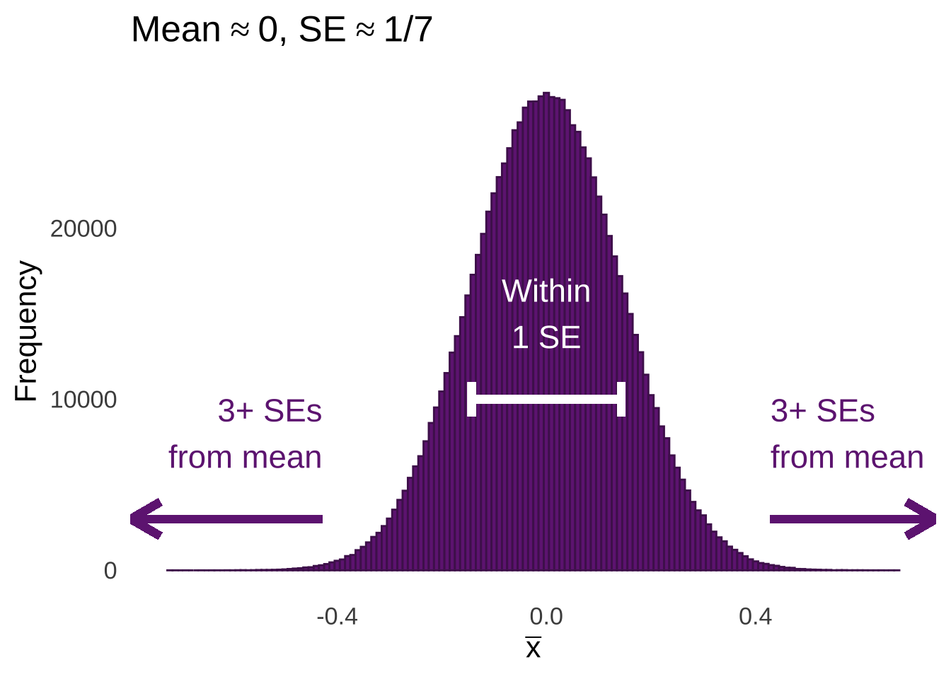
Figure 11.1: Histogram of the Means of 1,000,000 Samples of $n=49$ from a Standard Normal Distribution

The standard deviation of the sample means is the standard error (SE), which can be confusing since the it means that the standard error is a standard deviation with a standard deviation in the numerator of the formula to calculate it: $SE = SD/\sqrt{n}$. As difficult as it might be to get a handle on that tricky concept, it’s worth the work, as it helps us understand how the $t$-distribution and $t$-tests work.

As annotated in Figure 11.1, the majority of sample means are going to fall within 1 standard error of the mean of the sample means. Relatively few sample means are going to fall 3 or more standard errors from the mean. We can model the expectations of the distribution of sampling means using the $t$-distribution. For example, if we take all of the million sample means shown in Figure 11.1, and we divide each of them by their respective standard errors – that is, we take the standard deviation of the observations in the sample and divide by the square root of the number of observations $(sd/\sqrt{n})$, we will get the histogram of observed $t$-statistics on the top of Figure 11.2.

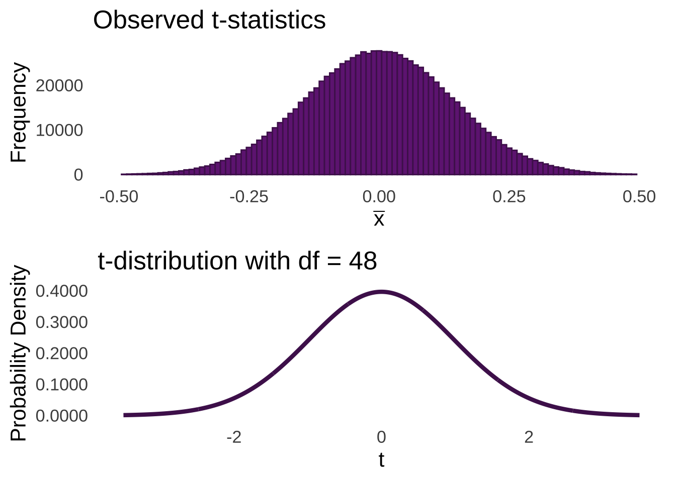
Figure 11.2: Histogram of $t$-statistics (top) and $t$-distribution with $df = 48$ (bottom)

Just as we can find areas under the curve of a normal distribution using $z$-scores given the mean and standard deviation of that normal distribution, we can use the number of standard errors from the mean of a $t$-distribution – which is zero – to determine areas under $t$ curves. And, like how $z$-scores represent the number of standard deviations a number is from the mean of a normal, the $t$-statistic is the number of $t$-distribution standard deviations – those are standard errors – an observed $t$ is from the mean.

To help describe what happens when sample means are drawn, please consider the two following examples that describe the process of using the smallest possible sample size – 1 – and the process of using the largest possible sample size – the size of the entire population, represented by approximately infinity – respectively.

If $n=1$, then the distribution of the sample means – which, since $n=1$, wouldn’t really be means so much as they would be the value of the samples themselves – would have a mean $\mu_{\bar{x}}=\mu$ and a standard deviation of $\frac{s^2_{\bar{x}}}{1}=\sigma^2$. Thus, each observation would be a sample from a normal distribution. As covered in the page on probability distributions, the probability of any one of those observations falling into a range is determined by the area under the normal curve. We know that the probability that a value sampled from a normal distribution is greater than the mean of the distribution is 50%. We know that the probability that a value sampled from a normal distribution is within one standard deviation of the mean is approximately 68%. And – this is important and we will come back to it several times – we know that the probability of sampling a value that is more than 1.645 standard deviations greater than the mean is approximately 5%:

pnorm(1.645, lower.tail=FALSE)

## [1] 0.04998491

the probability of sampling a value that is more than 1.645 standard deviations less than the mean is also approximately 5%:

pnorm(-1.645, lower.tail=TRUE)

## [1] 0.04998491

and that the probability that sampling a value that is either 1.96 standard deviations greater than or less than the mean is also approximately 5%:

pnorm(-1.96, lower.tail=TRUE)+pnorm(1.96, lower.tail=FALSE)

## [1] 0.04999579

In classical statistical tests, the null hypothesis implies that the sample being studied is an ordinary sample from a given distribution defined by certain parameters. The alternative hypothesis is that the sample being studied was taken from different distribution, such as a distribution of the same type but defined by different parameters (e.g., if the null hypothesis implies sampling from a standard normal distribution, the alternative hypothesis may be that the sample comes from another normal distribution with a different mean). We reject the null hypothesis if the cumulative likelihood of observing the observed data given that the null hypothesis is true is extraordinarily small. So, if we knew the mean and variance of a population and happened to observe a single value (or the mean of a single value, which is the value itself) that was several standard deviations away from the mean of the population that we assume under the null that we are sampling from, then we may conclude that we should reject the null hypothesis that that observation came from the null-hypothesis distribution in favor of the alternative hypothesis that the observation came from some other distribution.

Buddy (Will Ferrell) learning to reject the null hypothesis that he is sampled from a population of elves is a major plot point in the 2003 holiday classic Elf

Figure 11.3: Buddy (Will Ferrell) learning to reject the null hypothesis that he is sampled from a population of elves is a major plot point in the 2003 holiday classic Elf

If $n=\infty$, then the distribution of the sample means would have a mean equal to $\mu$ and a variance of $\sigma^2/\infty=0$¹⁸⁶. That means that if you could sample the entire population and take the mean, the mean you take would always be exactly the population mean. Thus, there would be no possible difference between the mean of the sample you take and the population mean – because the mean you calculated would necessarily be the population mean – and thus there would be no sampling error. In statistical terms, the end result would be a sampling error or standard error of 0.

With a standard error of 0, each mean we calculate would be expected to be the population mean. If we sampled an entire population and we did not calculate the expected population mean, then one of two things are true: either the expectation about the mean is wrong, or, more interestingly, we have sampled a different population than the one we expected.

11.1.2 One-sample $t$-test

In theory, the one-sample $t$-test assesses the difference between a sample mean and a hypothesized population mean. The idea is that a sample is taken, and the mean is measured. The variance of the sample data is used as an estimate of the population variance, so that the sample mean is considered to be – in the null hypothesis – one of the many possible means sampled from a normal distribution with the hypothesized population mean $\mu$ and a variance estimated from the sample variance ($\sigma^2 \approx s^2_{obs}$). The central limit theorem tells us that the distribution of the sample means – of which the mean of our observed data is assumed to be one in the null hypothesis – has a mean equal to the population mean ($\bar{x}=\mu$) and a variance equal to the population variance divided by the size of the sample ($\sigma^2_{\bar{x}}=\sigma^2/n$) and therefore a standard deviation equal to the population standard deviation divided by the square root of the size of the sample ($\sigma_{\bar{x}}=\sqrt{\sigma^2_{\bar{x}}}=\sigma/\sqrt{n}$, which is the standard error).

The $t$-statistic (or just $t$, if you’re into the whole brevity thing) measures how unusual the observed sample mean is from the hypothesized sample mean. It does so by measuring how far away the observed sample mean is from the hypothesized population mean in terms of standard errors (see the illustration in Figure 11.1).

The $t$-distribution models the distances of sample means from the hypothesized population mean in terms of standard errors as a function of the degrees of freedom ($df$) used in the calculation of those sample means (i.e., $n-1$). Smaller (in terms of $n$) samples from normal distributions are naturally more likely to be far away from the mean – there is greater sampling error for smaller samples – and the $t$-distribution reflects that by being more kurtotic when $df$ is small. That is, relative to $t$-distributions with large $df$, the tails of $t$-distributions for small $df$ are thicker and thus there are greater areas under the curve associated with extreme values of $t$ (see Figure 11.4, which is reproduced from probability distributions ).

Figure 11.4: The $t$ Distribution for Selected Values of $df$

Of course, it is possible to observe any mean value for a finite sample ¹⁸⁷ taken from a normal distribution. But, at some point, an observed sample mean can be so far from the mean and therefore the probability of observing a sample mean at least that far away is so unlikely that we reject the null hypothesis that the observed sample mean came from the population described in the null hypothesis. We reject the null hypothesis in favor of the alternative hypothesis that the sample came from some other population. We use the $t$-statistic to help us make that decision.

The observed $t$ that will help us make our decision is given by the formula:

\[t_{obs}=\frac{\bar{x}-\mu}{se}\]

where $\bar{x}$ is the observed sample mean, $\mu$ is the population mean posited in the null hypothesis, and $se$ is the standard error of the sample mean $s_{obs}/\sqrt{n}$, which approximates the standard deviation of all sample means of size $n$ taken from the hypothesized normal distribution $\sigma/\sqrt{n}$ (because we don’t really know what $\sigma$ is in the population).

As noted above, $\mu$ is the mean of a hypothetical population, but in practice it can be any number of interest. For example, if we were interested in whether the mean of a sample were significantly not equal to zero ($> 0,~< 0$, or $\ne 0$), we could put some variation of $\mu=0$ ($\le 0,~\ge 0$, or $=0$) in the null hypothesis to simulate what would happen if the population mean were 0? even if we aren’t really thinking about 0 in terms of a population mean.

11.1.2.0.1 One-sample $t$ Example

For our examples, let’s pretend that we are makers of large kitchen appliances. Let’s start by making freezers. First, we will have to learn how freezers work and how to build them.

Looks easy enough! Now we need to test our freezers. Let’s say we have built 10 freezers and we need to know that our sample of freezers produces temperatures that are significantly less than $0^{\circ} C$ ¹⁸⁸. Here, in degrees Celsius, are our observed data:

Freezer	Temperature ($^{\circ}C$)
1	-2.14
2	-0.80
3	-2.75
4	-2.58
5	-2.26
6	-2.46
7	-1.33
8	-2.85
9	-0.93
10	-2.01

Now we will use the six-step hypothesis testing procedure to test the scientific hypothesis that the mean of the internal temperatures of the freezers we built is significantly less than 0.

Oh, sorry, Nick Miller. First we must do the responsible thing and check the assumptions of the $t$-test. Since we have only one set of data (meaning we don’t have to worry about homoscedasticity), the only check we have to do is about normality:

shapiro.test(one.sample.data)

## 
##  Shapiro-Wilk normality test
## 
## data:  one.sample.data
## W = 0.89341, p-value = 0.1852

The Shapiro-Wilk test says we can continue to assume normality.

11.1.2.0.1.1 Six-Step Hypothesis Testing

Define null and alternative hypotheses.

For this freezer-temperature-measuring experiment, we are going to start by assuming that the mean of our observed temperatures is sampled from a normal distribution with a mean of 0. We don’t hypothesize a variance in this step: for now, the population variance is unknown (it will be estimated by the sample variance in the process of doing the $t$-test calculations in step 5 of the procedure).

Now, it will not do us any good – as freezer-makers – if the mean internal temperatures of our freezers is greater than $0^{\circ} C$. In this case, a point (or two-tailed) hypothesis will not do, because that would compel us to reject the null hypothesis if the mean were significantly less than or greater than $0^{\circ} C$. Instead we will use a directional (or one-tailed) hypothesis, where our null hypothesis is that we have sampled our mean freezer temperatures from a normal distribution of freezer temperatures with a population mean that is greater than or equal to 0 and our alternative hypothesis is that we have sampled our mean freezer temperatures from a normal distribution of freezer temperatures with a population mean that is less than 0.:

\[H_0:\mu \ge 0\] \[H_1: \mu <0\] 2. Define the type-I error (false-alarm) rate $\alpha$

Let’s say $\alpha=0.05$. Whatever.

Identify the statistical test to be used.

Since this is the one-sample $t$-test section of the page, let’s go with “one-sample $t$-test.”

Identify a rule for deciding between the null and alternative hypotheses

If the observed $t$ indicates that the cumulative likelihood of the observed $t$ or more extreme unobserved $t$ values is less than the type-I error rate (that is, if $p\le \alpha$), we will reject $H_0$ in favor of $H_1$.

We can determine whether $p \le \alpha$ in two different ways. First, we can directly compare the area under the $t$ curve for $t \le t_{obs}$ – which is $p$ because the null hypothesis is one-tailed and we will reject $H_0$ if $t$ is significantly less than the hypothesized population parameter $\mu$ – to $\alpha$. We can accomplish that fairly easily using software and that is what we will do (sorry for the spoiler).

The second way we can determine whether $p \le \alpha$ is by using critical values of $t$. A critical value table such as this one lists the values of $t$ for which $p$ is exactly $\alpha$ given the $df$ and whether the test is one-tailed or two-tailed. Any value of $t$ with an absolute value greater than the $t$ listed in the table for the given $\alpha$, $df$, and type of test necessarily has an associated $p$-value that is less than $\alpha$. The critical-value method is helpful if you (a) are in a stats class that doesn’t let you use R on quizzes and tests, (b) are stranded on a desert island with nothing but old stats books and for some reason need to conduct $t$-tests, and/or (c) live in 1955.

Obtain data and make calculations

The mean of the observed sample data is -2.01, and the standard deviation is 0.74. We incorporate the assumption that the observed standard deviation is our best guess for the population standard deviation in the equation to find the standard error:

\[se=\frac{sd_{obs}}{\sqrt{n}}\] although, honestly, if you don’t care much for the theoretical underpinning of the $t$ formula, it suffices to say the se is the sd divided by the square root of n.

Our null hypothesis indicated that the $\mu$ of the population was 0, so that’s what goes in the numerator of the $t_{obs}$ formula. Please note that it makes no difference at this point whether $H_0$ is $\mu \le 0$, $\mu =0$, or $\mu \ge 0$: the number associated with $\mu$ goes in the $t_{obs}$ formula; the equals sign or inequality sign comes into play in the interpretation of $t_{obs}$.

Thus, the observed $t$ is:

\[t=\frac{\bar{x}-\mu}{se}=\frac{-2.01-0}{0.23}=-8.59 \]

Make a decision

Now that we have an observed $t$, we must evaluate the cumulative likelihood of observing at least that $t$ in the direction(s) indicated by the type of test (one-tailed or two-tailed). Because the alternative hypothesis was that the population from which the sample was drawn had a mean less than 0, the relevant $p$-value is the cumulative likelihood of observing $t_{obs}$ or a lesser (more negative) $t$.

Because $n=10$ (there were 10 freezers for which we measured the internal temperature), $df=9$. We thus are looking for the lower-tail cumulative probability of $t \le t_{obs}$ given that $df=9$:

pt(-8.59, df=9, lower.tail=TRUE)

## [1] 6.241159e-06

That is a tiny $p$-value! It is much smaller than the $\alpha$ rate that we stipulated ($\alpha=0.05$). We reject $H_0.$

OR: the critical $t$ for $\alpha=0.05$ and $df=9$ for a one-tailed test is 1.833. The absolute value of $t_{obs}$ is $|-8.59|=8.59$, which is greater than the critical $t$. We reject $H_0$.

OR: we could have skipped all of this and just used R from the jump:

t.test(one.sample.data, mu=0, alternative = "less")

## 
##  One Sample t-test
## 
## data:  one.sample.data
## t = -8.5851, df = 9, p-value = 6.27e-06
## alternative hypothesis: true mean is less than 0
## 95 percent confidence interval:
##       -Inf -1.580833
## sample estimates:
## mean of x 
## -2.010017

but then we wouldn’t have learned as much.

11.1.3 Repeated-Measures $t$-test

The repeated-measures $t$-test is used when we have two measurements of the same things and we want to see if the mean of the differences for each thing is statistically significant. Mathematically, the repeated-measures $t$-test is the exact same thing as the one-sample $t$-test! The only special thing about it is that we get the sample of data by subtracting, for each observation, one measure from the other measure to get difference scores.

The repeated-measures $t$-test is just a one-sample $t$-test of difference scores.

Repeated measures compare individuals against themselves (or against matched individuals).

This reduces the effect of individual differences, for example:

In a memory experiment with different conditions, a repeated-measures design accounts for the fact that people naturally have different mnemonic capabilities

Differences related to different conditions are generally easier to detect, increasing power (more on that topic to come)

Another advantage of repeated-measures designs is that data can be collected under different conditions for the same participants, which saves the researcher from recruiting different participants for different conditions. The combination of reduced noise due to individual variation and collecting data from the same participants for different conditions means that repeated-measures designs are generally more efficient relative to similar independent-groups designs. And that’s not nothing: participant payment, animal subjects, and research time can be costly, and it’s generally good to do the best science one can given the resources at hand.

There are certain situations in which a repeated-measure design should be used with care. For example, some conditions may have order effects like fatigue or learning unrelated to the topic of the study. This is an example of an experimental design issue known as a confound: confounds tend to make it more difficult to interpret the results of a scientific study.

Also, there are certain situations in which a repeated-measure design cannot be used. Some research designs require making comparisons between completely different groups of people by the very nature of the research. Cognitive aging research, to name one field where that is frequently the case, often involves using younger adults as a comparison group for measuring cognition in older adults. Using a repeated-measures design for that kind of research would require recruiting young adults to participate, waiting several decades, and then asking those same, now-older adults to participate again. It’s highly impractical to do that in reality (unless you were working with a criminally unethical pharmaceutical company with access to a mystical beach that ages people a lifetime in 24 hours, which 1. you, personally, would not do and 2. was literally the plot to the 2021 movie Old), so that kind of research must use independent-groups designs.

11.1.3.0.1 Repeated-measures $t$ Example

To generate another example, let’s go back to our imaginary careers as makers of large kitchen appliances. This time, let’s make an oven. To test our oven, we will make 10 cakes, measuring the temperature each tin of batter in $^{\circ}C$ before they go into the oven and then measuring the temperature of each of the (hopefully) baked sponges after 45 minutes in the oven.

Here are the (made-up) data:

Cake	Pre-bake ($^{\circ} C$)	Post-bake ($^{\circ} C$)	Difference (Post $-$ Pre)
1	20.83	100.87	80.04
2	19.72	98.58	78.86
3	19.64	109.09	89.44
4	20.09	121.83	101.74
5	22.25	122.78	100.53
6	20.83	111.41	90.58
7	21.31	103.96	82.65
8	22.50	121.81	99.31
9	21.17	127.85	106.68
10	19.57	115.17	95.60

Once we have calculated the difference scores – which for convenience we will abbreviate with $d$ – we have no more use for the original paired data¹⁸⁹. The calculations proceed using $d$ precisely as they do for the observed data in the one-sample $t$-test.

11.1.3.1 Repeated Measures and Paired Samples

This is as good a time as any to pause and note that what I have been calling the repeated-measures $t$-test is often referred to as the paired-samples $t$-test. Either name is fine! What is important to note is that the measures in this test do not have to refer to the same individual. A paired sample could be identical twins. It could be pairs of animals that have been bred to be exactly the same with regard to some variable of interest (e.g., murine models). It could also be individuals that are matched on some demographic characteristic like age or level of education attained. From a statistical methods point of view, paired samples from different individuals are treated mathematically the same as are paired samples from the same individuals. Whether individuals are appropriately matched is a research methods issue.

Back to the math: the symbols and abbreviations we use are going to be specific to the repeated-measures $t$-test, but the formulas are going to be exactly the same. We calculate the observed $t$ for the repeated-measures test the same way as we calculated the observed $t$ for the one-samples test, but with assorted $d$’s in the formulas to remind us that we’re dealing with difference scores.

\[t_{obs}=\frac{\bar{d}-\mu_d}{se_d}\]

The null assumption is that we are drawing the sample of difference scores from a population of difference scores with a mean equal to $\mu_d$. The alternative hypothesis is that we are are sampling from a distribution with a different $\mu_d$.

So, now we are completely prepared to apply the six-step procedure to …

Oh, thanks, Han Solo! We have to test the normality of the differences:

shapiro.test(difference)

## 
##  Shapiro-Wilk normality test
## 
## data:  difference
## W = 0.93616, p-value = 0.5111

We can continue to assume that the differences are sampled from a normal distribution.

11.1.3.1.0.1 Six-step Hypothesis Testing

Identify the null and alternative hypotheses.

Let’s start with the scientific hypothesis that the oven will make the cakes warmer. Thus, we are going to assume a null that the oven makes the cakes no warmer or possibly less warm, with the alternative being that the $mu_d$ is any positive non-zero difference in the temperature of the cakes.

\[H_0: \mu_d \le 0\] \[H_1: \mu_d>0\] 2. Identify the type-I error (false alarm) rate.

Again, $\alpha=0.05$, a type-I error rate that might be described as…

So, this time, let’s instead use $\alpha=0.01$

Identify the statistical test to be used.

Repeated-measures $t$-test.

Identify a rule for deciding between the null and alternative hypotheses

If $p<\alpha$, which as noted for the one-sample $t$-test we can calculate with software or by consulting a critical-values table but really we’re just going to use software, reject $H_0$ in favor of $H_1$.

Obtain data and make calculations

The mean of the observed sample data is 92.54, and the standard deviation is 9.77. As for the one-sample test, we incorporate the assumption that the observed standard deviation of the differences is our best guess for the population standard deviation of the differences in the equation to find the standard error:

\[se_d=\frac{sd_{d(obs)}}{\sqrt{n}}\]

The observed $t$ for these data is:

\[t_{obs}=\frac{\bar{d}-\mu_d}{se_d}=\frac{92.54-0}{3.09}=29.97\]

Because the null hypothesis indicates that $\mu_d \le 0$, the $p$-value is the cumulative likelihood that of $t \ge t_{obs}$: an upper-tail probability. Thus, the observed $p$-value is:

pt(29.97, df=9, lower.tail=FALSE)

## [1] 1.252983e-10

The observed $p$-value is less than $\alpha=0.01$, so we reject the null hypothesis in favor of the alternative hypothesis: the population-level mean difference between pre-bake batter and post-bake sponge warmth is greater than 0.

Of course, we can save ourselves some time by using R. Please note that when using the t.test() command with two arrays (as we do with the repeated-measures test and will again with the independent-samples test), we need to note whether the samples are paired or not using the paired = TRUE/FALSE option.

t.test(postbake, prebake, mu=0, alternative="greater", paired=TRUE)

## 
##  Paired t-test
## 
## data:  postbake and prebake
## t = 29.966, df = 9, p-value = 1.255e-10
## alternative hypothesis: true mean difference is greater than 0
## 95 percent confidence interval:
##  86.88161      Inf
## sample estimates:
## mean difference 
##        92.54283

Based on this analysis, our ovens are in good working order.

But that result only tells us that the mean increase in temperature was significantly greater than 0. That is probably not good enough, even for imaginary makers of large kitchen appliances.

Suppose, then, that instead of using $\mu_d=0$ as our $H_0$, we used $\mu_d=90$ as our $H_0$. That would mean that we would be testing whether our ovens, on average, raise the temperature of our cakes by more than $90^{\circ}C$. We’ll skip all of the usual steps and just alter our R commands by changing the value of mu:

t.test(postbake, prebake, mu=90, alternative="greater", paired=TRUE)

## 
##  Paired t-test
## 
## data:  postbake and prebake
## t = 0.82337, df = 9, p-value = 0.2158
## alternative hypothesis: true mean difference is greater than 90
## 95 percent confidence interval:
##  86.88161      Inf
## sample estimates:
## mean difference 
##        92.54283

Thus, while the mean difference was greater than $90^{\circ}C$, it was not significantly so.

A couple of things to note for that. The first is the $p$-value changes because we changed the null hypothesis – more evidence that the $p$-value is not the probability of the data themselves. The other is that altering $\mu_d$ can be a helpful tool when assuming $\mu_d=0$ – which is the norm (and also the default in R if you leave out the mu= part of the t.test() command) – is not scientifically interesting.

11.1.4 Independent-Groups $t$-test

The last type of $t$-test is the independent-groups (or independent-samples) $t$-test. The independent-groups test is used when we have completely different samples. They don’t even have to be the same size.¹⁹⁰.

When groups are independent, the assumption is that they are drawn from different populations that have the same variance. The independent-samples $t$ is a measure of the difference of the means of the two groups. The distribution that the difference of the means is sampled from is not one of a single population but of the combination of the two populations.

The rules of linear combinations of random variables tell us that the difference of two normal distributions is a normal with a mean equal to the difference of the means of the two distributions and a variance equal to the sum of the means of the two distributions:

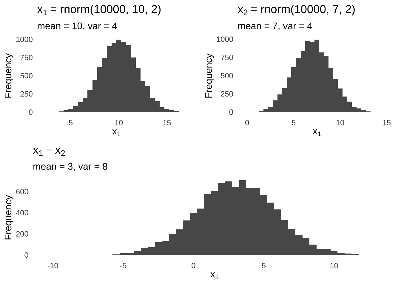
Figure 11.5: Linear (Subtractive) Combination of two Normal Distributions

And so the difference of the means is hypothesized to come from the combined distribution of the differences of the means of the two populations.

11.1.4.1 Pooled Variance

The variance of the population distributions that each sample comes from are assumed to be the same: that’s the homescedasticity assumption. When performing the one-sample and repeated-measures $t$-tests, we used the sample variances of the single sample and the difference scores, respectively, to estimate the populations from which those numbers came. But, with two groups, we will most likely have two sample variances (we could have the exact same sample variance in both groups, but that would be quite improbable). We can’t say that one sample comes from a population with a variance approximated by the variance of the that sample and that the other sample comes from a population with a variance approximated by the variance of the other sample: that would imply that the populations have different variances, and we can’t have that, now, can we?

Instead, we treat the two sample variances together as estimators of the common variance value of the two populations by calculating what is known as the pooled variance:

\[s^2_{pooled}=\frac{s^2_1(n_1-1)+s^2_2(n_2-1)}{n_1+n_2-2}\] The pooled variance, in practice, acts like a weighted average of the two sample variances: if the samples are of uneven size ($n1 \ne n_2$), by multiplying each sample variance by $n-1$, the variance of the larger sample is weighted more heavily than the variance of the smaller sample. In theory (in practice, too, I guess, but it’s a little harder to see), by multiplying the sample variances by their respective $n -1$, the pooled variance takes the numerator of the sample variances – the sums of squares (SS) for each observation – adds them together, and creates a new variance.

\[s^2_{pooled}=\frac{\sum(x_1-\bar{x}_1)^2+\sum(x_2-\bar{x}_2)^2}{n_1+n_2-2}\] The denominator of the pooled variance is the total degrees of freedom of the estimate: because there are two means involved in the calculation of the numerator – $\bar{x}_1$ to calculate the $SS$ of sample 1 and $\bar{x}_2$ to calculate the $SS$ of sample 2, the total $df$ is the total $n=n_1+n_2$ minus 2.

Now, our null assumption is that the difference of the means comes from a distribution generated by the combination of the two distributions from which the two means were respectively sampled with a hypothesized mean of the difference of means. The variance of that distribution is unknown at the time that the null and alternative hypotheses are determined¹⁹¹. When we do estimate that variance, it will be the pooled variance. And, when we apply the central limit theorem, we will use a standard error that – based on the rules of linear combinations – is a sum of the standard errors of each sampling procedure:

\[\bar{x1}-\bar{x2} \sim N \left( \mu_1 - \mu_2,~ \frac{\sigma^2}{n_1}+\frac{\sigma^2}{n_2}\right)\]

And therefore our formula for the observed $t$ for the independent-samples $t$-test is:

\[t_{obs}=\frac{\bar{x}_1-\bar{x}_2-\Delta}{\sqrt{\frac{s^2_{pooled}}{n_1}+\frac{s^2_{pooled}}{n_2}}}\] where $\Delta$ is the hypothesized mean of the null-distribution of the difference of means.

Please note: in practice, as with the repeated-measures $t$-test, researchers rarely use a non-zero value for the mean of the null distribution ($\mu_d$ in the case of the repeated-measures test; $\Delta$ in the case of the independent-samples test). Still, it’s there if we need it.

The $df$ that defines the $t$-distribution that our difference of sample means comes from is the sum of the degrees of freedom for each sample:

\[df=(n_1-1)+(n_2-1)=n_1+n_2-2\]

11.1.4.1.1 Independent-groups $t$ Example

Now, let’s think up another example to work through the math. In this case, let’s say we have expanded our kitchen-appliance-making operation to include small kitchen appliances, and we have made two models of toaster: the Mark I and the Mark II. Imagine, please, that we want to test if there is any difference in the time it takes each model to properly toast pieces of bread. We test 10 toasters of each model (here $n_1-n_2$ that’s doesn’t necessarily have to be true) of toaster and record the time it takes to finish the job:

Time to Toast (s)
Mark I	Mark II
4.72	9.19
7.40	11.44
3.50	9.64
3.85	12.09
4.47	10.80
4.09	12.71
6.34	10.04
3.30	9.06
7.13	6.31
4.99	9.44

We are now ready to test the hypothesis that there is any difference in the mean toasting time between the two models.

Oh, I almost forgot again! Thanks, Diana Ross! We have to test two assumptions for the independent-samples $t$-test: normality and homoscedasticity.

Mark.I.residuals<-Mark.I-mean(Mark.I)
Mark.II.residuals<-Mark.II-mean(Mark.II)

shapiro.test(c(Mark.I.residuals, Mark.II.residuals))

## 
##  Shapiro-Wilk normality test
## 
## data:  c(Mark.I.residuals, Mark.II.residuals)
## W = 0.94817, p-value = 0.3402

Good on normality!

model<-c(rep("Mark I", length(Mark.I)), rep("Mark II", length(Mark.II)))
times<-c(Mark.I, Mark.II)
independent.samples.df<-data.frame(model, times)
leveneTest(times~model, data=independent.samples.df)

## Levene's Test for Homogeneity of Variance (center = median)
##       Df F value Pr(>F)
## group  1   0.186 0.6714
##       18

And good on homoscedasticity, too!

Now, we may proceed with the six-step procedure.

Identify the null and alternative hypotheses.

We are looking in this case for evidence that either the Mark I toaster or the Mark II toaster is faster than the other. Logically, that means that we are interested in whether the difference between the mean toasting times is significantly different from 0. Thus, we are going to assume a null that indicates no difference between the population mean of Mark I toaster times and the population mean of Mark II toaster times.

\[H_0: \bar{x}_1- \bar{x}_2 = 0\] \[H_1: \bar{x}_1 - \bar{x}_2 \ne 0\] 2. Identify the type-I error (false alarm) rate.

The type-I error rate we used for the repeated-measures example – $\alpha=0.01$ – felt good. Let’s use that again.

Identify the statistical test to be used.

Independent-groups $t$-test.

Identify a rule for deciding between the null and alternative hypotheses

If $p<\alpha$, which again we can calculate with software or by consulting a critical-values table but there’s no need to get tables involved here in the year 2020, reject $H_0$ in favor of $H_1$.

Obtain data and make calculations

The mean of the Mark I sample is 4.98, and the variance is 2.19. The mean of the Mark II sample is 10.07, and the variance is 3.33.

The pooled variance for the two samples is:

\[s^2_{pooled}=\frac{s^2_1(n_1-1)+s^2_2(n_2-1)}{n_1+n_2-2}=\frac{2.19(10-1)+3.33(10-1)}{10+10-2}=2.76\]

The observed $t$ for these data is:

\[t_{obs}=\frac{\bar{x}_1-\bar{x}_2-\Delta}{\sqrt{\frac{s^2_{pooled}}{n_1}+\frac{s^2_{pooled}}{n_2}}}=\frac{4.98-10.07-0}{\sqrt{\frac{2.76}{10}+\frac{2.76}{10}}}=-6.86\]

Because this is a two-tailed test, the $p$-value is the sum of the cumulative likelihood of $t\le-|t_{obs}|$ or $t\ge|t_{obs}|$ – that is, the sum of the lower-tail probability that a $t$ could be less than or equal to the negative version of $t_{obs}$ and the upper-tail probability that a $t$ could be greater than or equal to the positive version of $t_{obs}$:

pt(-6.86, df=18, lower.tail=TRUE)+pt(6.86, df=18, lower.tail=FALSE)

## [1] 2.033668e-06

And all that matches what we could have done much more quickly and easily with the t.test() command. Note in the following code that paired=FALSE – otherwise, R would run a repeated-measures $t$-test – and that we have included the option var.equal=TRUE, which indicates that homoscedasticity is assumed. Assuming homoscedasticity is not the default option in R: more on that below.

t.test(Mark.I, Mark.II, mu=0, paired=FALSE, alternative="two.sided", var.equal=TRUE)

## 
##  Two Sample t-test
## 
## data:  Mark.I and Mark.II
## t = -6.8552, df = 18, p-value = 2.053e-06
## alternative hypothesis: true difference in means is not equal to 0
## 95 percent confidence interval:
##  -6.654528 -3.532506
## sample estimates:
## mean of x mean of y 
##  4.979966 10.073482

11.1.4.2 Welch’s $t$-test

The default option for the t.test() command when paired=FALSE is indicated is var.equal=FALSE. That means that without instructing the software to assume homoscedasticity, the default is to assume different variances. This default test is known as Welch’s $t$-test. Welch’s test differs from the traditional, homoscedasticity-assuming $t$-test in two ways:

The pooled variance is replaced by separate population variance estimates based on the sample variances. The denominator for Welch’s $t$ is therefore:

\[\sqrt{\frac{s^2_1}{n^1}+\frac{s^2_2}{n^2}}\] 2. The degrees of freedom of the $t$-distribution are adjusted to compensate for the differences in variance. The degrees of freedom for the Welch’s test are not $n_1+n_2-2$, but rather:

\[df\approx\frac{\left( \frac{s^2_1}{n_1}+\frac{s^2_2}{n_2} \right)^2}{\frac{s^4_1}{n_1^2(n_1-1)}+\frac{s^4_2}{n_2^2(n_2-1)}}\]

Really, what you need to know there is that the Welch’s test uses a different $ than the traditional independent-samples test.

Repeating, then, the analysis of the toasters with var.equal=TRUE removed, the result of the Welch test is:

t.test(Mark.I, Mark.II, mu=0, paired=FALSE, alternative="two.sided")

## 
##  Welch Two Sample t-test
## 
## data:  Mark.I and Mark.II
## t = -6.8552, df = 17.27, p-value = 2.566e-06
## alternative hypothesis: true difference in means is not equal to 0
## 95 percent confidence interval:
##  -6.659274 -3.527760
## sample estimates:
## mean of x mean of y 
##  4.979966 10.073482

Note that for these data where homoscedasticity was observed, the $t_obs$ is the same. The $df$ is a non-integer value, but close to the value of $df=18$ for the traditional independent-samples test, and the $p$-value is essentially the same.

The advantage of Welch’s test is that it accounts for possible violations of homoscedasticity. I don’t really see a downside except that you may have to explain it a tiny bit in a write-up of your results.

11.1.4.2.1 Notes on the $t$-test

Although I chose one or the other for each of the above examples, any type of $t$-test can be either a one-tailed test or a two-tailed test. The direction of the hypothesis depends only on the nature of the question one is trying to answer, not on the structure of the data.
Some advice for one-tailed tests: always be sure to keep track of your signs. For the one-tailed test, that is relatively easy: keep in mind whether you are testing whether the sample mean is supposed to be greater than the null value or less than the null value. For the repeated-measures and independent-groups tests, be careful which values you are subtracting from which. Which measurement you subtract from which in the repeated-measures test and which mean you subtract from which in the independent-groups test is arbitrary. However, it can be shocking if, for example, you expect scores to increase from one measurement to another and they appear to decrease, but only because you subtracted what was supposed to be bigger from what was supposed to be smaller (or vice versa).
Related to note 2: assuming that the proper subtractions have been made, if you have a directional hypothesis and the result is in the wrong direction, it cannot be statistically significant. If, for example, the null hypothesis is $\mu \le 0$ and the $t$ value is negative, then one cannot reject the null hypothesis no matter how big the magnitude of $t$. An experiment testing a new drug with a directional hypothesis that the drug will make things better is not successful if the drug makes things waaaaaaaay worse.

11.1.5 $t$-tests and Regression

Check this out:

Let’s run a linear regression on our toaster data where the predicted variable ($y$) is toasting time and the predictor variable ($x$) is toaster model. Note the $t$-value on the “modelMark.II” line:

toaster.long<-data.frame(model=c(rep("Mark.I", 10), rep("Mark.II", 10)), times=c(Mark.I, Mark.II))

summary(lm(times~model, data=toaster.long))

## 
## Call:
## lm(formula = times ~ model, data = toaster.long)
## 
## Residuals:
##     Min      1Q  Median      3Q     Max 
## -3.7588 -0.9213 -0.3457  1.3621  2.6393 
## 
## Coefficients:
##              Estimate Std. Error t value Pr(>|t|)    
## (Intercept)    4.9800     0.5254   9.479 2.02e-08 ***
## modelMark.II   5.0935     0.7430   6.855 2.05e-06 ***
## ---
## Signif. codes:  0 '***' 0.001 '**' 0.01 '*' 0.05 '.' 0.1 ' ' 1
## 
## Residual standard error: 1.661 on 18 degrees of freedom
## Multiple R-squared:  0.7231, Adjusted R-squared:  0.7077 
## F-statistic: 46.99 on 1 and 18 DF,  p-value: 2.053e-06

That $t$-value is the same as the $t$ that we got from the $t$-test (but with the sign reversed), and the $p$-value is the same as well. The $t$-test is a special case of regression: we’ll come back to that later.

11.2 Nonparametric Tests of the Differences Between Two Things

Nonparametric Tests evaluate the pattern of observed results rather than the numeric descriptors (e.g., summary statistics like the mean and the standard deviation) of the results. Where a parametric test might evaluate the cumulative likelihood (given the null hypothesis, of course) that people in a study improved on average on a measure following treatment, a nonparametric test might take the same data and evaluate the cumulative likelihood that $x$ out of $n$ people improved on the same measure following treatment.

Three examples of nonparametric tests were covered in correlation and regression: the correlation of ranks $\rho$, the concordance-based correlation $\tau$, and the categorical correlation $\gamma$. In each of those tests, it is not the relative values of paired observations with regard to the mean and standard deviation of the variables but the relative patterns of paired observations.

11.2.1 Nonparametric Tests for 2 Independent Groups

11.2.1.1 The $\chi^2$ Test of Statistical Independence

Statistical Independence refers to a state where the patterns of the observed data do not depend on the number of possibilities for the data to be arranged. That means that there is no relationship between the number of categories that a set of datapoints can be classified into and the probability that the datapoints will be classified in a particular way. By contrast, statistical dependence is a state where there is a relationship between the possible data structure and the observed data structure.

The $\chi^2$ test of statistical independence takes statistical dependence as its null hypothesis and statistical independence as its alternative hypothesis. It is essentially the same test as the $\chi^2$ goodness-of-fit test, but used for a wider variety of applied statistical inference (that is, beyond evaluating goodness-of-fit). $\chi^2$ tests of statistical independence can be categorized by the number of factors being analyzed in a given test: in this section, we will talk about the one factor case – one-way $\chi^2$ tests – and the two factor case – two-way $\chi^2$ tests.

11.2.1.1.1 One-way $\chi^2$ Test of Statistical Independence

In the one-way $\chi^2$ test, statistical independence is determined on the basis of the number of possible categories for the data.¹⁹²

To help illustrate, please imagine that 100 people who are interested in ordering food open up a major third-party delivery service website and see the following:

There are two choices, neither of which is accompanied by any type of description. We would expect an approximately equal number of the 100 hungry people to pick each option. Given that there is no compelling reason to choose one over the other, the choice responses of the people are likely to be statistically dependent on the number of choices. We would expect approximately $\frac{n}{2}=50$ people to order from Restaurant A and approximately $\frac{n}{2}=50$ people to order from Restaurant B: statistical dependence means we can guess based solely on the possible options.

Now, let’s say our 100 hypothetical hungry people open the same third-party food-delivery website and instead see these options:

Given that the titles of each restaurant are properly descriptive and not ironic, this set of options would suggest that people’s choices will not depend solely on the number of options. The choice responses of the 100 Grubhub customers would likely follow a non-random pattern. Their choices would likely be statistically independent of the number of possible options.

As in the goodness-of-fit test, the $\chi^2$ test of statistical independence uses an observed $\chi^2$ test statistic that is calculated based on observed frequencies ($f_o$, although it’s sometimes abbreviated $O_f$) and on _expected frequencies ($f_e$, sometimes $E_f$):

\[\chi^2_{obs}=\sum_1^k \frac{(f_o-f_e)^2}{f_e}\] where $k$ is the number of categories or cells that the data can fall into. For the one-way test, the expected frequencies for each cell are the total number of observations divided by the number of cells:

\[f_e=\frac{n}{k}.\] The expected frequencies do not have to be integers! In fact, unless the number of observations is a perfect multiple of the number of cells, they will not be.

11.2.1.1.2 Degrees of Freedom

The degrees of freedom ($df$, sometimes abbreviated with the Greek letter $\nu$ [“nu”]) for the one-way $\chi^2$ test is the number of cells $k$ minus 1:

\[df=k-1\]

Generally speaking, the degrees of freedom for a set of frequencies (as we have in the data that can be analyzed with the $\chi^2$ test) are the number of cells whose count can change while maintaining the same marginal frequency. For a one-way, two-cell table of data with $A$ observations in the first cell and $B$ observations in the second cell, the marginal frequency is $A+B$:

cell	cell	margin
A	B	A+B

thus, we can think of the marginal frequencies as totals on the margins of tables comprised of cells. If we know $A$, and the marginal frequency $A+B$ is fixed, then we know $B$ by subtraction. The observed frequency of $A$ can change, and then (given fixed $A+B$) we would know $B$; $B$ could change, and then we would know $A$. We cannot freely change both $A$ and $B$ while keeping $A+B$ constant; thus, there is 1 degree of freedom for the two-cell case.

As covered in probability distributions, $df$ is the sufficient statistic for the $\chi^2$ distribution: it determines both the mean ($df$) and the variance ($2df$). Thus, the $df$ are all we need to know to calculate the area under the $\chi^2$ curve at or above the observed $\chi^2$ statistic: the cumulative likelihood of the observed or more extreme unobserved $\chi^2$ values. The $\chi^2$ distribution is a one-tailed distribution and the $\chi^2$ test is a one-tailed test (the alternative hypothesis of statistical independence is a binary thing – there is no such thing as either negative or positive statistical independence), so that upper-tail probability is all we need to know.

As the $\chi^2$ test is a classical inferential procedure (albeit one that makes an inference on the pattern of observed data and no inference on any given population-level parameters), it observes the traditional six-step procedure. The null hypothesis of the $\chi^2$ test – as noted above – is always that there is statistical dependence and the alternative hypothesis is always that there is statistical independence. Whatever specific form dependence and independence take, respectively, depends (no pun intended) on the situation being analyzed. The $\alpha$-rate is set a priori, the test statistic is a $\chi^2$ value with $k-1$ degrees of freedom, and the null hypothesis will be rejected if $p \le \alpha$.

To make the calculations, it is often convenient to keep track of the expected and observed frequencies in a table resembling this one:


$f_e$		$f_e$
	$f_0$		$f_0$

We then determine whether the cumulative likelihood of the observed $\chi^2$ value or more extreme $\chi^2$ values given the null hypothesis of statistical dependence – mathematically, statistical dependence looks like $\chi^2\approx 0$ – is less than or equal to the predetermined $\alpha$ rate either by using a table of $\chi^2$ quantiles.

Let’s work through an example using the fictional choices of 100 hypothetical people between the made-up restaurants Dan’s Delicious Dishes and Homicidal Harry’s House of Literal Poison. Suppose 77 people choose to order from Dan’s and 23 people choose to order from Homicidal Harry’s. Under the null hypothesis of statistical dependence, we would expect an equal frequency in each cell: 50 for Dan’s and 50 for Homicidal Harry’s:

fe1<-c("$f_e=50$", "")
fo1<-c("", "$f_0=77$")
fe2<-c("$f_e=50$", "")
fo2<-c("", "$f_0=23$")


kable(data.frame(fe1, fo1, fe2, fo2), "html", booktabs=TRUE, escape=FALSE, col.names = c("", "", "", "")) %>% 
  kable_styling() %>% 
  row_spec(1, italic=TRUE, font_size="small")%>% 
  row_spec(2, font_size = "large") %>% 
  add_header_above(c("Dan's"=2, "Harry's"=2)) %>% 
  column_spec(2, border_right = TRUE)

Dan’s		Harry’s

$f_e=50$		$f_e=50$
	$f_0=77$		$f_0=23$

The observed $\chi^2$ statistic is:

\[\chi^2_{obs}=\sum_i^k \frac{(f_o-f_e)^2}{f_e}=\frac{(77-50)^2}{50}+\frac{(23-50)^2}{50}=14.58+14.58=29.16\] The cumulative probability of $\chi^2\ge 29.16$ for a $\chi^2$ distribution with $df=1$ is:

pchisq(29.16, df=1, lower.tail=FALSE)

## [1] 6.66409e-08

which is smaller than an $\alpha$ of 0.05, or an $\alpha$ of 0.01, or really any $\alpha$ that we would choose. Thus, we reject the null hypothesis of statistical dependence in favor of the alternative of statistical independence. In terms of the example: we reject the null hypothesis that people are equally likely to order from Dan’s Delicious Dishes or from Homicidal Harry’s House of Literal Poison in favor of the alternative that there is a statistically significant difference in people’s choices.

To perform the $\chi^2$ test in R is blessedly more simple:

chisq.test(c(77, 23))

## 
##  Chi-squared test for given probabilities
## 
## data:  c(77, 23)
## X-squared = 29.16, df = 1, p-value = 6.664e-08

11.2.1.1.3 Relationship with the Binomial

Now, you might be thinking:

Wait a minute … the two-cell one-way $\chi^2$ test seems an awful lot like a binomial probability problem. What if we treated these data as binomial with $s$ as the frequency of one cell and $f$ as the frequency of the other with a null hypothesis of $\pi=0.5$?

And it is very impressive that you might be thinking that, because the answer is:

A one-way two-cell $\chi^2$ test will result in approximately the same $p$-value as $p(s \ge s_{obs} |\pi=0.5, N)$, where $s$ is the greater of the two observed frequencies (or $p(s \le s_{obs}| \pi=0.5, N)$ where $s$ is the lesser of the two observed frequencies). In fact, the binomial test is the more accurate of the two methods – the $\chi^2$ is more of an approximation – but the difference is largely negligible.

To demonstrate, we can use the data from the above example regarding fine dining choices:

pbinom(76, 100, 0.5, lower.tail=FALSE)

## [1] 2.75679e-08

The difference between the $p$-value from the binomial and from the $\chi^2$ is about $4 \times 10^8$. That’s real small!

11.2.1.1.4 Using Continuous Data with the $\chi^2$ Test

The $\chi^2$ test assesses categories of data, but that doesn’t necessarily mean that the data themselves have to be categorical. In the goodness-of-fit version, for example, numbers in a dataset were categorized by their values: we can do the same for the test of statistical independence.

Suppose a statistics class of 12 students received the following grades – $\{85, 85, 92, 92, 93, 95, 95, 96, 97, 98, 99, 100 \}$ – and we wanted to know if their grade breakdown was significantly different from a 50-50 split between A’s and B’s. We could do a one-sample $t$-test based on the null hypothesis that $\mu=90$. Or, we could use a $\chi^2$ test where the expected frequencies reflect an equal number of students scoring above and below 90:

fe1<-c("$f_e=6$", "")
fo1<-c("", "$f_0=2$")
fe2<-c("$f_e=6$", "")
fo2<-c("", "$f_0=12$")


kable(data.frame(fe1, fo1, fe2, fo2), "html", booktabs=TRUE, escape=FALSE, col.names = c("", "", "", "")) %>% 
  kable_styling() %>% 
  row_spec(1, italic=TRUE, font_size="small")%>% 
  row_spec(2, font_size = "large") %>% 
  add_header_above(c("B's"=2, "A's"=2))

B’s		A’s

$f_e=6$		$f_e=6$
	$f_0=2$		$f_0=12$

The observed $\chi^2$ statistic would be:

\[\chi^2_{obs}=\frac{(2-6)^2}{6}+\frac{(10-6)^2}{6}=5.33\] The $p$-value – given that $df=1$ – would be 0.021, which would be considered significant at the $\alpha=0.05$ level.

11.2.1.1.5 The Two-Way $\chi^2$ Test

Often in statistical analysis we are interested in examining multiple factors to see if there is a relationship between things, like exposure and mutation, attitudes and actions, study and recall. The two-way version of the $\chi^2$ test of statistical independence analyzes patterns in category membership for two different factors. To illustrate: imagine we have a survey comprising two binary-choice responses: people can answer $0$ or $1$ to Question 1 and they can answer $2$ or $3$ to Question 2. We can organize their responses into a $2 \times 2$ ($rows \times columns$) table known as a contingency table, where the responses to each question – the marginal frequencies of responses – are broken down contingent upon their answers to the other question.¹⁹³

		Question 2
		2	3	Margins
Question 1	0	$A$	$B$	$A+B$
Question 1	1	$C$	$D$	$C+D$
	Margins	$A+C$	$B+D$	$n$

Statistical independence in the one-way $\chi^2$ test was determined as a function of the number of possible options. Statistical independence in the two-way $\chi^2$ test suggests that the two factors are independent of each other, that is, that the number of possibilities for one factor are unrelated to the categorization of another factor.

11.2.1.1.6 Degrees of Freedom for the 2-way $\chi^2$ Test

Just as the degrees of freedom for the one-way $\chi^2$ test were the number of cells in which the frequency was allowed to vary while keeping the margin total the same, the degrees of freedom for the two-way $\chi^2$ test are the number of cells that are free to vary in frequency while keeping both sets of margins – the margins for each factor – the same. Thus, we have a set of $df$ for the rows of a contingency table and a set of $df$ for the columns of a contingency table, and the total $df$ is the product of the two:

\[df=(k_{rows}-1)\times (k_{columns}-1))\]

11.2.1.1.7 Expected Frequencies for the 2-way $\chi^2$ Test

Unlike in the one-way test, the expected frequencies across cells in the two-way $\chi^2$ test do not need to be equal: in most cases, they aren’t. It is possible – and not at all uncommon – for the different response levels of each factor to have different frequencies, which the two-way test accounts for. The expected frequencies instead are proportionally equal given the marginal frequencies. In the arrangment in the table above, for example, we do not expect $A$, $B$, $C$, and $D$ to be equal to each other but we do expect $A$ and $B$ to be _proportional to $A+C$ and $A+D$, respectively; for $A$ and $C$ to be proportional to $A+B$ and $C+D$, respectively; etc.

Thus, the expected frequency for each cell in a 2-way contingency table is:

\[f_e=n \times row~proportion \times column~proportion\] For example, let’s say that we asked 140 people a 2-question survey:

Is a hot dog a sandwich?
Does a straw have one hole or two?

and that these are the observed frequencies:

		How many holes does a straw have?
		1	2	Margins
Is a hot dog a sandwich?	Yes	40	10	50
Is a hot dog a sandwich?	No	20	70	90
	Margins	60	80	140

The expected frequencies, generated by the formula $f_e=n \times row~proportion \times column~proportion$ for each cell, are presented in the following table above and to the left of their respective observed frequencies:

		How many holes does a straw have?
			1		2	Margins
Is a hot dog a sandwich?	Yes	21.43		28.57
	Yes		40		10	50
	No	38.57		51.43
	No		20		70	90
	Margins		60		80	140

Note, for example, that the expected number of people to say “no” to the hot dog question and “1” to the straw question is greater than the expected number of people to say “yes” to the hot dog question and “1” to the straw question, even though the opposite was observed. That is because more people overall said “no” to the hot dog question, so proportionally we expect greater number of responses associated with either answer to the other question among those people who (correctly) said that a hot dog is not a sandwich.

The observed $\chi^2$ value for the above data is:

\[\chi^2_{obs} (1)=\frac{(40-21.43)^2}{21.43}+\frac{(10-28.57)^2}{28.57}+\frac{(20-38.57)^2}{38.57}+\frac{(70-51.43)^2}{51.43}=43.81\]

The associated $p$-value is:

pchisq(65.27, df=1, lower.tail=FALSE)

## [1] 6.530801e-16

which is smaller than any reasonable $\alpha$-rate, so we reject the null hypothesis that there is no relationship between people’s responses to the hot dog question and the straw question.

To perform the one-way $\chi^2$ test in R, we used the command chisq.test() with a vector of values inside the parentheses. The two-way test has an added dimension, so instead of a vector, we enter a matrix:

matrix(c(40, 20, 10, 70), nrow=2)

##      [,1] [,2]
## [1,]   40   10
## [2,]   20   70

When calculating the $\chi^2$ test on a $2 \times 2$ matrix, R defaults to applying Yates’s Continuity Correction. Personally, I think you can skip it, although it doesn’t seem to do too much harm. We can turn off that default with the option correct=FALSE.

chisq.test(matrix(c(40, 20, 10, 70), nrow=2), correct=FALSE)

## 
##  Pearson's Chi-squared test
## 
## data:  matrix(c(40, 20, 10, 70), nrow = 2)
## X-squared = 43.815, df = 1, p-value = 3.61e-11

11.2.1.1.8 Beyond the 2-way $\chi^2$ Test

Having had a blast with the one-way $\chi^2$ test and the time of one’s life with the two-way $\chi^2$ test, one might be tempted to add increasing dimensions to the $\chi^2$ test…

Such things are mathematically doable, but not terribly advisable for two main reasons:

Adding dimensions increases the number of cells exponentially: a three-way test involves $x \times y \times z$ cells, a four-way test involved $x \times y \times z \times q$ cells, etc. In turn, that means that an exponentially rising number of observations is needed for reasonable analysis of the data. In a world of limited resources, that can be a dealbreaker.
The larger problem is one of scientific interpretation. It is relatively straightforward to explain a scientific hypothesis involving the statistical independence of two factors. It is far more difficult to generate a meaningful scientific hypothesis involving the statistical independence of three or more factors, especially if it turns out – as it can – that the $\chi^2$ test indicates statistical independence of all of the factors but not some subsets of the factors or vice versa.

So, the official recommendation here is to use factorial analyses other than the $\chi^2$ test should more than two factors apply to a scientific hypothesis.

11.2.1.1.8.1 Dealing with small $f_e$

As noted in our previous encounter with the $\chi^2$ statistic, the only requirement for the $\chi^2$ test is that $f_e\ge 5$. If the structure of observed data are such that you would use a 1-way $\chi^2$ test except for the problem of $f_e < 5$, we can instead treat the data as binomial, testing the cumulative likelihood of $s \ge s_{obs}$ given that $\pi=0.5$. If the structure indicate a 2-way $\chi^2$ test but $f_e$ is too small, then we can use the Exact Test.

11.2.1.2 Exact Test

The Exact Test – technically known as Fisher’s Exact Test but since he was a historically shitty person I see no problem dropping his name from the title – is an alternative to the $\chi^2$ test of statisical independence to use when there is:

a $2 \times 2$ data structure and
inadequate $f_e$ per cell to use the $\chi^2$ test.

The exact test returns the cumulative likelihood of a given pattern of data given that the marginal totals remain constant. To illustrate how the exact test returns probabilities, please consider the following labels for a $2 \times 2$ contingency table:

	Factor 2		Margins

Factor 1	$A$	$B$	$A+B$
Factor 1	$C$	$D$	$C+D$
Margins	$A+C$	$B+D$	$n$

First, let’s consider the number of possible combinations for the row margins. Given that there are $n$ observations, the number of combinations of observations that could put $A+B$ of those observations in the top row – and therefore $C+D$ observations in the second row – is given by:

\[nCr=\frac{n!}{(A+B)!(n-(A+B))!}=\frac{n!}{(A+B)!(C+D)!}\]

Next, let’s consider the arrangement of the row observations into column observations. The number of combinations of observations that lead to $A$ observations in the first column is $A+C$ things combined $A$ at a time – $_{A+C}C_A$ – and the number of combinations of observations that lead to $B$ observations in the second column is $B+D$ things combined $B$ at a time – $_{B+D}C_B$. Therefore, there are a total of $_{A+C}C_A \times _{B+D}C_B$ possible combinations that lead to the observed $A$ (and thus $C$ because $A+C$ is constant) and the observed $B$ (and thus $D$ because $B+D$ is constant), and the formula:

\[\frac{(A+C)!}{A!C!} \times \frac{(B+D)!}{B!D!}=\frac{(A+C)!(B+D)!}{A!B!C!D!}\] describes the number of possible ways to get the observed arrangement of $A$, $B$, $C$, and $D$. Because, as noted above, there are $\frac{n!}{(A+B)!(C+D)!}$ total possible arrangements of the data, probability of the observed arrangement is the number of ways to get the observed arrangement divided by the total possible number of arrangements:

\[p(configuration)=\frac{\frac{(A+C)!(B+D)!}{A!B!C!D!}}{\frac{n!}{(A+B)!(C+D)!}}=\frac{(A+B)!(C+D)!(A+C)!(B+D)!}{n!A!B!C!D!}\]

The $p$-value for the Exact Test is the cumulative likelihood of all configurations that are as extreme or more extreme than the observed configuration.¹⁹⁴

The extremity of configurations is determined by the magnitude of the difference between each pair of observations that constitute a marginal frequency: that is: the difference between $A$ and $B$, the difference between $C$ and $D$, the difference between $A$ and $C$, and the difference between $B$ and $D$. The most extreme cases occur when the members of one group are split entirely into one of the cross-tabulated groups, for example: if $A+B=A$ because all members of the $A+B$ group are in $A$ and 0 are in $B$. Less extreme cases occur when the members of one group are indifferent to the cross-tabulated groups, for example: if $A+B\approx 2A \approx 2B$ because $A \approx B$.

Consider the following three examples: two with patterns of data suggesting no relationship between the two factors and another with a pattern of data suggesting a significant relationship between the two factors.

Example 1: An ordinary pattern of data

		How many holes does a straw have?
		1	2	Margins
Is a hot dog a sandwich?	Yes	4	3	7
Is a hot dog a sandwich?	No	4	4	8
	Margins	8	7	15

In this example, an approximately equal number of responses are given to both questions: 7 people say a hot dog is a sandwich, 8 say it is not; 8 people say a straw has 1 hole, 7 say it has 2. Further, the cross-tabulation of the two answers shows that people who give either answer to one question have no apparent tendencies to give a particular answer to another question: the people who say a hot dog is a sandwich are about even-odds to say a straw has 1 hole or 2; people who say a hot dog is not a sandwich are exactly even-odds to say a straw has 1 or 2 holes (and vice versa).

The probability of the observed pattern of responses is:

\[p=\frac{(A+B)!(C+D)!(A+C)!(B+D)!}{n!A!B!C!D!}=\frac{7!8!8!7!}{15!4!3!4!4!}=0.381\] Given that $p=0.381$ is greater than any reasonable $\alpha$-rate, calculating just the probability of the observed pattern is enough to know that the null hypothesis will not be rejected and we will continue to assume no relationship between the responses to the two questions. However, since this is more-or-less a textbook, and because there is no better place than a textbook than to do things by the book, we will examine the patterns that are more extreme than the observed data given that the margins remain constant.

Here is one such more extreme pattern:

		How many holes does a straw have?
		1	2	Margins
Is a hot dog a sandwich?	Yes	5	2	7
Is a hot dog a sandwich?	No	3	5	8
	Margins	8	7	15

Note that the margins in the above table are the same as in the first table: $A+B=7$, $C+D=8$, $A+C=8$, and $B+D$=7. However, the cell counts that make up those margins are a little more lopsided: $A$ and $D$ are a bit larger than $B$ and $C$. The probability of this pattern is:

\[p=\frac{(A+B)!(C+D)!(A+C)!(B+D)!}{n!A!B!C!D!}=\frac{7!8!8!7!}{15!5!2!3!5!}=0.183\] The next most extreme pattern is:

		How many holes does a straw have?
		1	2	Margins
Is a hot dog a sandwich?	Yes	6	1	7
Is a hot dog a sandwich?	No	2	6	8
	Margins	8	7	15

The probability of this pattern is:

\[p=\frac{(A+B)!(C+D)!(A+C)!(B+D)!}{n!A!B!C!D!}=\frac{7!8!8!7!}{15!6!1!2!6!}=0.03\] Finally, the most extreme pattern possible given that the margins are constant is:

		How many holes does a straw have?
		1	2	Margins
Is a hot dog a sandwich?	Yes	6	1	7
Is a hot dog a sandwich?	No	2	6	8
	Margins	8	7	15

(A good sign that you have the most extreme pattern is that there is a 0 in at least one of the cells.)

The probability of this pattern is:

\[p=\frac{(A+B)!(C+D)!(A+C)!(B+D)!}{n!A!B!C!D!}=\frac{7!8!8!7!}{15!6!1!2!6!}=0.0012\] The sum of the probabilities for the observed pattern and all more extreme unobserved patterns:

\[p=0.381+0.183+0.030+0.001=0.596\] is the $p$-value for a directional (one-tailed) hypothesis that there will be $A$ or more observations in the $A$ cell. That sort of test is helpful if we have a hypothesis about the odds ratio associated with observations being in the $A$ cell, but isn’t super-relevant to the kinds of problems we are investigating here. More pertinent is the two-tailed test (of a point hypothesis) that there is any relationship between the two factors. To get that, we would repeat the above procedure the other way (switching values such that the $B$ and $C$ cells get bigger) and add all of the probabilities.

But, that’s a little too much work, even going by the book. Modern technology provides us with an easier solution. Using R, we can arrange the observed the data into a matrix:

exact.example.1<-matrix(c(4, 4, 3, 4), nrow=2)
exact.example.1

##      [,1] [,2]
## [1,]    4    3
## [2,]    4    4

and then run an exact test with the base command fisher.test(). To check our math from above, we can use the option alternative = "greater":

fisher.test(exact.example.1, alternative="greater")

## 
##  Fisher's Exact Test for Count Data
## 
## data:  exact.example.1
## p-value = 0.5952
## alternative hypothesis: true odds ratio is greater than 1
## 95 percent confidence interval:
##  0.1602859       Inf
## sample estimates:
## odds ratio 
##   1.307924

To test the two-tailed hypothesis, we can either use the option alternative = "two.sided" or – since two.sided is the default, just leave it out:

fisher.test(exact.example.1)

## 
##  Fisher's Exact Test for Count Data
## 
## data:  exact.example.1
## p-value = 1
## alternative hypothesis: true odds ratio is not equal to 1
## 95 percent confidence interval:
##   0.1164956 15.9072636
## sample estimates:
## odds ratio 
##   1.307924

Either way, the $p$-value is greater than any $\alpha$-rate we might want to use, so we continue to assume the null hypothesis that there is no relationship between the factors, in this case: that responses on the two questions are independent.

Example 2: A Pattern Indicating a Significant Relationship

		How many holes does a straw have?
		1	2	Margins
Is a hot dog a sandwich?	Yes	7	0	7
Is a hot dog a sandwich?	No	0	8	8
	Margins	7	8	15

This table represents the most extreme possible patterns of responses: everybody who said a hot dog was a sandwich also said that a straw has one hole, and nobody who said a hot dog was a sandwich said that a straw has two holes. There is no more possible extreme on the other side of the responses: if $A$ equalled 0 and $B$ equalled 7, then $C$ would have to be 7 and $D$ would have to be 1 to keep the margins the same.

Thus, for this pattern, the one-tailed $p$-value for the observed data and the two-tailed $p$-value are both the probability of the observed pattern:

exact.example.2<-matrix(c(7, 0, 0, 8), nrow=2)
exact.example.2

##      [,1] [,2]
## [1,]    7    0
## [2,]    0    8

fisher.test(exact.example.2)

## 
##  Fisher's Exact Test for Count Data
## 
## data:  exact.example.2
## p-value = 0.0001554
## alternative hypothesis: true odds ratio is not equal to 1
## 95 percent confidence interval:
##  5.83681     Inf
## sample estimates:
## odds ratio 
##        Inf

Example 3: A Pattern That Looks Extreme But Does Not Represent a Significant Relationship

Finally, let’s look at a pattern that seems to be as extreme as it possibly can be:

		How many holes does a straw have?
		1	2	Margins
Is a hot dog a sandwich?	Yes	7	8	15
Is a hot dog a sandwich?	No	0	0	0
	Margins	7	8	15

In this observed pattern of responses, there is a big difference between $A$ and $C$ and between $B$ and $D$. Crucially, though, there is hardly any difference between $A$ and $B$ or between $C$ and $D$. Even though there are no moves we can make that maintain the same marginal numbers, the pattern here is one where the responses for one question don’t depend at all on the responses for the other question: in this set of data, people are split on the straw question but nobody regardless of their answer to the straw question thinks that a hot dog is a sandwich¹⁹⁵. The $p$-value for the Exact Test accounts for the lack of dependency between the responses:

exact.example.3<-matrix(c(7, 0, 8, 0), nrow=2)
fisher.test(exact.example.3)

## 
##  Fisher's Exact Test for Count Data
## 
## data:  exact.example.3
## p-value = 1
## alternative hypothesis: true odds ratio is not equal to 1
## 95 percent confidence interval:
##    0 Inf
## sample estimates:
## odds ratio 
##          0

11.2.1.2.1 Median Test

The core concept of the median test is: are there more values that are greater than the overall median of the data than there are from one sample than from another sample? The idea is that if one sample of data has values that tend to be bigger than values in another sample – with the overall median observation as the guide to what is bigger and what is smaller – then there is a difference between the two samples.

The median test arranges the observed data into two categories: less than the median and greater than the median. Values that are equal to the median can be part of either category – it’s largely a matter of preference – so those category designations, more precisely, can either be less than or equal to the median/greater than the median or less than the median/greater than or equal to the median (the difference will only be noticeable in rare, borderline situations). When those binary categories are crossed with the membership of values in one of two samples, the result is a $2 \times 2$ contingency table: precisely the kind of thing we analyze with a $\chi^2$ test of statistical independence or – if $f_e$ is too small for the $\chi^2$ test – the Exact Test.

To illustrate the median test, we will use two examples: one an example of data that do not differ with respect to the median value between groups and another where the values do differ between groups with respect to the overall median.

Example 1: an Ordinary Configuration

Imagine, if you will, the following data are observed for the dependent variable in an experiment with a control condition and an experimental condition:

Median = 57
	Control Condition	Experimental Condition
Below Median ($<57$	2, 12, 18, 23, 31, 35	4, 15, 16, 28, 44, 49
At or Above Median ($\ge 57$)	57, 63, 63, 66, 66, 69, 75	64, 67, 77, 84, 84, 85, 98, 100, 102

A plot of the above data with annotations for the overall median value (57, in this case), illustrates the similarity of the two groups:

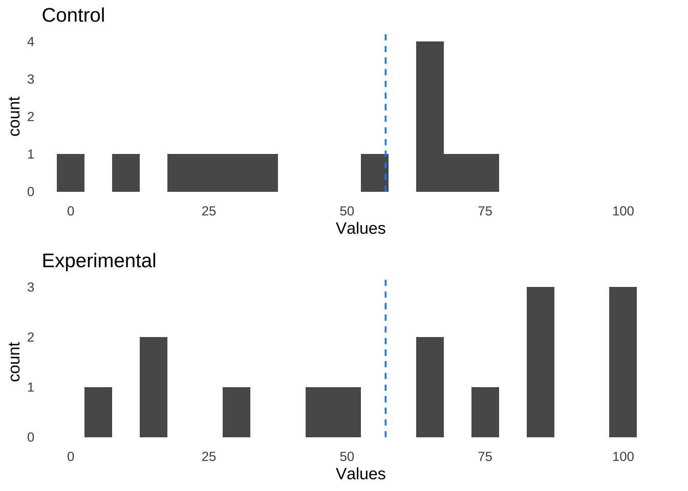
Figure 11.6: Control Group and Experimental Group Data Similar to Each Other With Respect to the Overall Median of 57

Tallying up how many values are below the median and how many values are greater than or equal to the median in each group results in the following contingency table:

	Control	Experimental
$<57$	7	9
$\ge 57$	6	6

This arrangement lends itself nicely to a $\chi^2$ test of statistical independence with $df=1$:

\[\chi^2_{obs}(1)=\frac{(7-7.43)^2}{7.43}+\frac{(9-8.57)^2}{8.57}+\frac{(6-5.57)^2}{5.57}+\frac{(6-6.43)^2}{6.43}=0.1077, p = 0.743\]

The results of the $\chi^2$ test lead to the continued assumption of independence between between category (less than/greater than or equal to the median) and condition (control/experimental), which we would interpret as there being no effect of being in the control vs. the experimental group with regard to the dependent variable.

Example 2: A Special Configuration

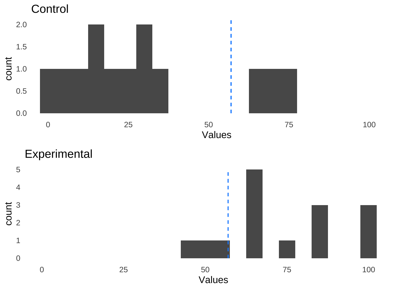
In the second example, there are more observed values in the control condition that are less than the median than there are values greater than or equal to the median and more observed values in the experimental condition that are greater than or equal to the median than there are values less than the median:

Median = 57
	Control Condition	Experimental Condition
Below Median ($<57$)	2, 4, 12, 15, 16, 18, 23, 28, 31, 35	44, 49
At or Above Median ($\ge 57$)	66, 69, 75	57, 63, 63, 64, 66, 67, 77, 84, 84, 85, 98, 100, 102

Counting up how many values in each group are either less than or greater than or equal to the overall median gives the following contingency table:

	Control	Experimental
$<57$	10	2
$\ge 57$	3	13

which in turn leads to the following $\chi^2$ test result:

\[\chi^2_{obs}(1)=\frac{(3-7.43)^2}{7.43}+\frac{(13-8.57)^2}{8.57}+\frac{(10-5.57)^2}{5.57}+\frac{(2-6.43)^2}{6.43}=11.50, p < .001\]

11.2.2 The Wilcoxon Mann-Whitney $U$ Test

The Wilcoxon Mann-Whitney $U$ Test ¹⁹⁶is a more powerful nonparametric test of differences between independent groups than the Median Test. It is a direct comparison of the overlap of the values in two different datasets: in the most extreme case, all of the values in one group of data are greater than all of the values in the other group; if there is no difference between groups, there will be subtantial overlap between the two groups.

The null hypothesis for the Wilcoxon-Mann-Whitney $U$ test is that if we make an observation X from population A and an observation Y from population B, it is equally probable that X is greater than Y and that Y is greater than X:

\[H_0: p(X>Y)=p(Y>X)\]

and thus, the alternative hypothesis is that the probability that X is greater than Y is not equal to the probability that Y is greater than X (or vice versa: the designation of X and Y is arbitrary):

\[H_1: p(X>Y)\ne p(Y>X)\] The Wilcoxon-Mann-Whitney test statistic $U$ is calculated thus:

Given two conditions A and B (in real life they will have real-life names like “control condition” or “experimental condition”):

For each value in A, count how many values in B are smaller. Call this count $U_A$
For each value in B, count how many values in A are smaller. Call this count $U_B$
The lesser of $U_A$ and $U_B$ is $U$
Test the significance of $U$ using tables for small $n$, normal approximation for large $n$.

Note: the Wilcoxon-Mann-Whitney test ignores ties. If there are tied data, the observed $p$-value will be imprecise (still usable, just imprecise).

For example, imagine the following data – which suggest negligible differences between the two group – are observed:

11.2.2.0.1 Example of an Ordinary Configuration:

Control Condition	Experimental Condition
12, 22, 38, 42, 50	14, 25, 40, 44, 48

We can arrange the data in overall rank order and mark whether each datapoint comes from the Control (C) condition or the Experimental (E) condition:

Configuration of Observed Data
C	E	C	E	C	E	C	E	E	C
12	14	22	25	38	40	42	44	48	50

To calculate $U_C$ (for the control condition), we take the total number of values from the experimental condition that are smaller than each value of the control condition. There are 0 experimental-condition values smaller than the smallest value in the control condition (12), 1 that is smaller than the second-smallest value (22), 2 that are smaller than the third-smallest value (38), 3 that are smaller than 42, and 5 that are smaller than 50 for a total of $U_C=11$.

To calculate $U_E$ (for the experimental condition), we take the total number of values for the control condition that are smaller than each value of the experimental condition. There is 1 control-condition value smaller than the smallest experimental-condition value (14), 2 that are smaller than 25, 3 that are smaller than 40, 4 that are smaller than 44, and also 4 that are smaller than 48 for a total of $U_E=14$.

The smaller of $U_C$ and $U_E$ is $U_C=11$. Given that $n$ for both groups is 5, we can use a critical value table to see that 11 is greater than the critical value for a two-tailed test¹⁹⁷

We can also use software to calculate both the $U$ statistic and the $p$-value (there is also a paired-samples version of the Wilcoxon test called the Wilcoxon Signed Rank Test; as with the t.test() command, we get the independent-samples version with the option paired=TRUE:

control<-c(12, 22, 38, 42, 50)
experimental<-c(14, 25, 40, 44, 48)
wilcox.test(control, experimental, paired=FALSE)

## 
##  Wilcoxon rank sum exact test
## 
## data:  control and experimental
## W = 11, p-value = 0.8413
## alternative hypothesis: true location shift is not equal to 0

Oh, and R calls $U$ “W.” Pretty sure that’s for consistency with the output for the Wilcoxon Signed Rank Test.

The following data provide an example of a pattern that does suggest a difference between groups:

Control Condition	Experimental Condition
12, 14, 22, 25, 40	38, 42, 44, 48, 50

Configuration of Observed Data
C	C	C	C	E	C	E	E	E	E
12	14	22	25	38	40	42	44	48	50

For these data, there is only one value of the experimental condition that is smaller than any of the control-condition values (38 is smaller than 40), and 24 control-condition values that are smaller than experimental-condition values, so the $U$ statistic is equal to $U_C=1$:

control<-c(12, 14, 22, 25, 40)
experimental<-c(38, 42, 44, 48, 50)
wilcox.test(control, experimental, paired=FALSE)

## 
##  Wilcoxon rank sum exact test
## 
## data:  control and experimental
## W = 1, p-value = 0.01587
## alternative hypothesis: true location shift is not equal to 0

11.2.2.0.1.1 Normal Approximation:

If either sample has $n>20$, then the following formulas can be used to calculate a $z$-score that then can be used to get a $p$-value based on areas under the normal curve

\[\mu=\frac{n_1n_2}{2}\]

\[\sigma=\sqrt{\frac{n_1n_2(n_1+n_2+1)}{12}}\]

\[z=\frac{U-\mu}{\sigma}\]

But: that is a pre-software problem that we don’t face anymore.

11.2.2.1 Randomization (Permutation) Test

The randomization test is the most powerful nonparametric test for analyzing two independent samples of scale data.¹⁹⁸ The central idea of the randomization test is: of all the possible patterns of the data, how unusual is the observed pattern?

11.2.2.1.1 Example of an Ordinary Configuration:

Control Condition	Experimental Condition
12, 22, 38, 42, 50	14, 25, 40, 44, 48

There are 126 patterns that are as likely or less likely than this one.

\[Number~of~possible~permutations=\frac{n!}{r!(n-r)!}=\frac{10!}{5!(10-5)!}=252\]

\[p=\frac{126}{252}=.5, n.s.\]

11.2.2.1.2 Example of a Special Configuration:

Control Condition	Experimental Condition
12, 14, 22, 25, 40	38, 42, 44, 48, 50

This is the second-least likely possible pattern of the observed data (the least likely would be if 38 and 40 switched places).

\[p=\frac{2}{252}=.0079\]

To find the $p$-value for the randomization test, follow this algorithm:

Calculate the possible number of patterns in the observed data using the combinatorial formula¹⁹⁹
Assign positive signs to one group of the data and negative signs to the other
Find the sum of the signed data. Call this sum $D$.
Switch the signs on the data and sum again to find all possible patterns that lead to greater absolute values of $D$
Take the count of patterns that lead to equal or greater absolute values of $D$
Divide the count in step 5, add 1 for the observed pattern, and divide by the possible number of patterns calculated in step 1 to find the $p$-value

Control:negative	Experimental: positive
-12, -14, -22, -25, -40	38, 42, 44, 48, 50

\[D=−12−14−22−25−40+38+42+44+48+50=109\]

Are there more extreme patterns? Only one: switch the signs of $38$ (from the experimental condition) and $40$ (from the control condition)

\[D=−12−14−22−25−38+40+42+44+48+50=113\]

In this example, there are two possible combinations that are equal to or more extreme than the observed pattern.

There are 252 possible patterns of the data

The $p$-value of the observed pattern is $2/252=.0079$

$\therefore$ we reject the null hypothesis.

11.2.3 Nonparametric Tests for 2 Paired Groups

11.2.3.1 McNemar’s Test

McNemar’s test is a repeated-measures test for categorical (or categorized continuous) data. Just as the repeated-measures $t$-test measures the difference between two measures of the same entities (participants, animal subjects, etc.), McNemar’s test measures categorical change among two entities. Given two possible categorical states – for example: healthy and unwell, in favor and opposed, passing and failing – of which each entity can exist in either at the times of the two different measurements, McNemar’s test is a way to analyze the differences in the two measures as a function of how much change happened between the two measurements.

To perform the test, the data are arranged thusly (with generic labels for the two possible states and the two measurements):

		Measure 2
		State 2	State 1
Measure 1	State 1	A	B
Measure 1	State 2	C	D

In this arrangement, $A$ and $D$ represent changes in the state: $A$ represents the count of entities that went from State 1 in the first measurement to State 2 in the second, and $D$ represents the count that went from State 2 in the first measurement to State 1 in the second.

If $A+D> 20$, the differences are measured using McNemar’s $\chi^2$:

\[\chi^2_{obs}(1)=\frac{(A-D)^2}{A+D}\] The larger the difference between $A$ and $D$ – normalized by the sum $A+D$ – the bigger the difference between the two measurements. And, by extension, larger differences between $A$ and $D$ indicate how important whatever came between the two measurements (a treatment, an intervention, an exposure, etc.) was.

If $A+D\le20$, use binomial likelihood formula with $\pi=0.5$:

\[p(s \ge \max(A, D)|\pi=0.5, N=A+D)=\sum \frac{N!}{A!D!}\pi^{\max(A, D)}(1-\pi)^{\min(A, D)}\] to be clear: given that $\pi=0.5$ for the McNemar test and the binomial distribution is therefore symmetrical, the equation:

\[p(s \le \min(A, D)|\pi=0.5, N=A+D)=\sum \frac{N!}{A!D!}\pi^{\min(A, D)}(1-\pi)^{\max(A, D)}\]

will produce the same result.

For example, please imagine students in a driver’s education class are given a pre-test on the rules of right-of-way before taking the class and a post-test on the same content after taking the class. In the first set of example data, there is little evidence of difference indicated between the two conditions by the observed data ($n=54$):

		Post-test
		Fail	Pass
Pre-test	Pass	15	8
Pre-test	Fail	16	15

In this example, 15 students pass the pre-test and fail the post-test, and another 15 students fail the pre-test and pass the post-test. There are 24 students whose performance remains in the same category for both the pre- and post-test (8 pass both; 16 fail both) – those data provide no evidence either was as to the efficacy of the class.

The McNemar $\chi^2$ statistic – which we can use instead of the binomial because $15+15>20$, is:

\[McNemar~\chi^2(1)=\frac{(15-15)^2}{15+15}=0\] Which we don’t need to bother finding the $p$-value for: it’s not in any way possibly significant.

In the second example data set, there is evidence that the class does something:

		Post-test
		Fail	Pass
Pre-test 1	Pass	25	8
Pre-test 1	Fail	16	5

In these data, 25 students pass the pre-test but fail the post-test, and 5 fail the pre-test but pass the post-test. The McNemar $\chi^2$ statistic for this set of data is:

\[McNemar~\chi^2(1)=\frac{(25-5)^2}{25+5}=\frac{400}{30}=13.3\] Measured in terms of a $\chi^2$ distribution with 1 degree of freedom – this might have been intuitable from the $2 \times 2$ structure of the data, but the McNemar is always a $df=1$ situation – the observed $p$-value is:

pchisq(13.3, df=1, lower.tail=FALSE)

## [1] 0.0002654061

and so we would reject the null hypothesis had we set $\alpha=0.5$, or $\alpha=0.01$, or even $\alpha=0.001$. Based on these data, there is a significant effect of the class.

Reviewing these particular data, we could further interpret the results as indicating that the class makes students significantly worse at knowing the rules of the road. Which in turn suggests that this driver’s ed class was taught in the Commonwealth of Massachusetts.

Conducting the McNemar test in R is nearly identical to conducting the $\chi^2$ test in R. The one thing to keep in mind is that the mcnemar.test() command expects the cells to be compared to be on the reverse diagonal:

\[\begin{bmatrix} B & A\\ D & C \end{bmatrix}\]

but, it’s not much trouble to just switch the columns. Also, you may want to – as with the $\chi^2$ test – turn off the continuity correction with the option correct=FALSE:

mcnemar.test(matrix(c(8, 5, 25, 16), nrow=2), correct=FALSE)

## 
##  McNemar's Chi-squared test
## 
## data:  matrix(c(8, 5, 25, 16), nrow = 2)
## McNemar's chi-squared = 13.333, df = 1, p-value = 0.0002607

11.2.3.2 Sign (Binomial) Test

The Sign test, like McNemar’s test, is a measure of categorical change over 2 repeated measures. In the case of the sign test, the categories are, specifically: positive changes and negative changes. It takes the sign of the observed changes in the dependent variable – positive or negative; zeroes are ignored – and treats them as binomial events with $\pi=0.5$. In other words, the sign test treats whether the difference between conditions is positive or negative as a coin flip. For that reason, the sign test is often referred to as the binomial test, which is fine, but I think there are so many things (including several on this page alone) that can be statistically analyzed with the binomial likelihood function that that name can be a little confusing.

The $p$-value for a binomial test is the cumulative binomial probability of the number of positive values or negative values observed given the total number of trials that didn’t end up as ties and $\pi=0.5$. If there is a one-tailed hypothesis with an alternative that indicates that more of the changes will be positive, then that cumulative probability is the probability of getting at least as many positive changes out of the non-zero differences; if there is a one-tailed hypothesis with an alternative that indicates that more of the changes will be negative, then the cumulative probability is that of getting at least as many positive changes out of the non-zero differences. If the hypothesis is two-tailed, then the $p$-value is the sum of the probability of getting the smaller of the number of the positive changes and the negative changes or fewer plus the probability of getting $n$ – that number or greater (since the sign test is a binomial with $\pi$=0.5, that’s more easily computed by taking the cumulative probability of the smaller of the positive count and the negative count or fewer and multiplying it by two).

The following is an example data set in which positive changes are roughly as frequent as negative changes: a data set for which we would expect our sign test analysis to come up with a non-significant result.

Observation	Before	After	Difference	Sign of Difference
1	1	3	2	$+$
2	8	5	-3	$-$
3	0	2	2	$+$
4	0	-1	-1	$-$
5	1	1	0	$=$
6	3	-5	-8	$-$
7	3	7	4	$+$
8	3	362	359	$+$
9	5	1	-4	$-$
10	6	0	-6	$-$
11	5	10	5	$+$

Let’s use a one-tailed test with a null hypothesis that the number of positive changes will be greater than or equal to the number of negative changes ($\pi \ge 0.5$) and an alternative hypothesis that the number of positive changes will be less than the number of negative changes ($\pi < 0.5$) Of the $n=11$ observations, one had a difference score of 0. We throw that out. Of the rest, there are 5 positive differences and 5 negative differences. Therefore, we calculate the cumulative binomial probability of 5 or fewer successes in 10 trials with $\pi=0.5$:

pbinom(5, 10, 0.5)

## [1] 0.6230469

and find that the changes are not significant. The software solution in R is fairly straightforward:

binom.test(5, 10, 0.5, alternative="less")

## 
##  Exact binomial test
## 
## data:  5 and 10
## number of successes = 5, number of trials = 10, p-value = 0.623
## alternative hypothesis: true probability of success is less than 0.5
## 95 percent confidence interval:
##  0.0000000 0.7775589
## sample estimates:
## probability of success 
##                    0.5

For a counterexample, let’s use the following example data where there are many more negative changes than positive changes:

Observation	Before	After	Difference	Sign of Difference
1	1	3	2	$+$
2	8	5	-3	$-$
3	0	-2	-2	$-$
4	0	-1	-1	$-$
5	1	1	0	$=$
6	3	-5	-8	$-$
7	3	-7	-10	$-$
8	3	-362	-365	$-$
9	5	-1	-6	$-$
10	6	0	-6	$-$
11	5	-10	-15	$-$

In this case, there is still 1 observation with no change between measurements: we’ll toss that and we are left with 10 observations with changes: 9 negative and 1 positive. This time, we will use a 2-tailed test. The sign test $p$-value is therefore (keeping in mind that for an upper-tail pbinom, we enter $s-1$ for $s$):

pbinom(1, 10, 0.5)+pbinom(8, 10, 0.5, lower.tail=FALSE)

## [1] 0.02148438

Using binom.test() with the option alternative="two.sided" gives us the same result:

binom.test(1, 10, 0.5, alternative="two.sided")

## 
##  Exact binomial test
## 
## data:  1 and 10
## number of successes = 1, number of trials = 10, p-value = 0.02148
## alternative hypothesis: true probability of success is not equal to 0.5
## 95 percent confidence interval:
##  0.002528579 0.445016117
## sample estimates:
## probability of success 
##                    0.1

11.2.3.3 Wilcoxon Signed-Rank Test

The Wilcoxon Signed-Rank Test is the paired-samples version of the Wilcoxon-Mann-Whitney $U$ test. It operates in much the same way as the sign test, but it is more powerful because it takes into account the magnitude of the ranks of the differences. That is, a small negative difference means less in the calculation of the test statistic than a large negative difference, and likewise a small positive difference means less than a large positive difference. Thus, significant values of the Wilcoxon test statistic $W$ come from combinations of large and frequent positive shifts or combinations of large and frequent negative shifts.

To calculate the Wilcoxon $W$ statistic, we begin by taking differences (as we do with all of the tests with two repeated measures). We note the sign of the difference: positive or negative, and as in the sign test throwing out the ties. We also rank the magnitude of the differences from smallest (1) to largest ($n$). If there are ties in the differences, each tied score gets the average rank of the untied rank above and the untied rank below the tie cluster. For example, if a set of differences is $\{10, 20, 20, 30\}$, $10$ is the smallest value and gets rank 1; $40$ is the largest value and gets rank 4, and the two $20's$ get the average rank $\frac{1+4}{2}=2.5$, thus, the ranks would be $\{1, 2.5, 2.5, 4\}$.

We then combine the ranks and the signs to get the signed-ranks. For example, if the observed differences were $\{10, 20, 20, 30\}$, then the signed ranks would be $\{1, 2.5, 2.5, 4\}$. If the observed differences were $\{-10, -20, -20, -30\}$, then the signed ranks would be $\{-1, -2.5, -2.5, -4\}$: the ranks are based on magnitude (or, absolute value), so even though $-30$ is the least of the four numbers, $-10$ is the smallest in terms of magnitude.

knitr::include_graphics("images/magnitude.gif")

Figure 11.7: Magnitude

For the one-tailed test, $W$ is equal to the sum of the positive ranks. For the two-tailed test, the $W$ statistic is the greater of the sum of the magnitudes of the positive ranks and the sum of the magnitudes of the negative ranks. If we denote the sum of the positive ranks as $T^+$ and the sum of the negative ranks as $T^-$, then we can write the $W$ formulaw like this:

\[One-tailed~W=\max(T^+, T^-)\] \[Two-tailed~W=T^+\] To demonstrate the Wilcoxon signed-rank test in action, we can re-use the examples from the sign test. First, the dataset that indicates no significant effect:

Observation	Before	After	Difference	Sign of Difference	Rank	Signed Rank
1	1	3	-2	$-$	2.5	$-$ 2.5
2	8	5	3	$+$	4.0	$+$ 4
3	0	2	-2	$-$	2.5	$-$ 2.5
4	0	-1	1	$+$	1.0	$+$ 1
5	1	1	0	$=$	0.0	0
6	3	-5	8	$+$	9.0	$+$ 9
7	3	7	-4	$-$	5.5	$-$ 5.5
8	3	362	-359	$-$	10.0	$-$ 10
9	5	1	4	$+$	5.5	$+$ 5.5
10	6	0	6	$+$	8.0	$+$ 8
11	5	10	-5	$-$	7.0	$-$ 7

The sum of the positive signed-rank magnitudes is:

\[T^+=2.5+2.5+5.5+10+7=27.5\] which is equal to $W$ if we want the one-tailed test.

The sum of the negative signed-rank magnitudes is (note: we drop the negative signs to get the sum of the magnitudes):

\[T^-=4+1+9+5.5+8=27.5\] and thus for the two-tailed test:

\[W=\max(32.5, 32.5)=32.5\] To test the significance of $W$ statistics where $n\le30$, we can look up a critical value in a table.

If $n>30$, there is a normal approximation that will produce a $z$-score; the area under the normal curve beyond which will give the approximate $p$-value for the $W$ statistic:

\[z=\frac{W-\frac{n(n+1)}{4}}{\sqrt{\frac{n(n+1)(2n+1)}{24}-\frac{1}{2}\sum_{i=1}^g t_j(t_j-1)(t_j+1)}}\] where $g$ is the number of tie clusters in the ranks and $t_j$ is the number of ties in each cluster $j$. I honestly hope you never use that formula.

We can just use the wilcox.test() command with the paired=TRUE option.

wilcox.test(Before, After, paired=TRUE, correct = FALSE)

## 
##  Wilcoxon signed rank test
## 
## data:  Before and After
## V = 27.5, p-value = 1
## alternative hypothesis: true location shift is not equal to 0

I have no idea why R decides to call $W$ $V$.

Now let’s apply the same procedure to a dataset that indicates evidence of a difference between the Before and After measures:

Observation	Before	After	Difference	Sign of Difference	Rank	Signed Rank
1	1	3	-2	$-$	2.5	$-$ 2.5
2	8	5	3	$+$	4.0	$+$ 4
3	0	-2	2	$+$	2.5	$+$ 2.5
4	0	-1	1	$+$	1.0	$+$ 1
5	1	1	0	$=$	0.0	0
6	3	-5	8	$+$	7.0	$+$ 7
7	3	-7	10	$+$	8.0	$+$ 8
8	3	-362	365	$+$	10.0	$+$ 10
9	5	-1	6	$+$	5.5	$+$ 5.5
10	6	0	6	$+$	5.5	$+$ 5.5
11	5	-10	15	$+$	9.0	$+$ 9

The sum of the positive signed-rank magnitudes (there is only one) is:

\[T^+=2.5\]

The sum of the negative signed-rank magnitudes is (again: we drop the negative signs to get the sum of the magnitudes):

\[T^-=4+2.5+1+7+8+10+5.5+5.5+9=52.5\] and thus:

\[One-tailed~W=T^+\]

\[Two-tailed~W=\max(2.5, 52.5)=52.5\]

To test the significance of $W$, we can just take the easier and more sensible route straight to the software solution:

wilcox.test(Before, After, paired=TRUE)

## 
##  Wilcoxon signed rank test with continuity correction
## 
## data:  Before and After
## V = 52.5, p-value = 0.0124
## alternative hypothesis: true location shift is not equal to 0

Note: R will always return the value of $T^+$ as the test statistic, but the $p$-value is unaffected by the difference.

11.2.3.4 Repeated-Measures Randomization Test

The repeated-measures randomization test works on the same basic principle as the independent-groups randomization test: the observed scores – in the case of the repeated-measures test, the observed differences – are taken as a given. The question is how unusual is the arrangement of those scores. If the magnitudes of the positive changes and the negative changes are about the same, then the pattern is nothing special. If the magnitudes of the positive changes are in total much larger than the magnitudes of the negative changes or vice versa, then the pattern is unusual and there is likely a significant effect.

The repeated-measures randomization test is also similar in principle to the Wilcoxon Signed-Rank Test, in that it examines the relative sizes of the negative and the positive changes, but different in that it deals with the observed magnitudes of the data themselves rather than their ranks.

Again, we assume that the observed magnitudes of the differences are given, but that the sign on each difference can vary. That means that number of possible permutations of the data are $2^n$ (or, more accurately, $2^{n-the number of ties}$, because we ignore any ties). The paired-samples randomization test is an analysis of how many patterns are as extreme as or more extreme than the observed pattern; the $p$-value is the number of such patterns divided by the $2^n$ possible patterns.

To illustrate, please imagine that we observed the following data in a two-condition psychological experiment:

Participant<-1:7
Condition1<-c(13,42,9,5,6,8,18)

Condition2<-c(5,36,2,0,9,7,9)
Difference<-Condition1-Condition2

kable(data.frame(Participant, Condition1, Condition2, Difference), "html", booktabs=TRUE, align=c("c", "c", "c", "c"), col.names=c("Participant", "Condition 1", "Condition 2", "Difference")) %>% 
  kable_styling()

Participant	Condition 1	Condition 2	Difference
1	13	5	8
2	42	36	6
3	9	2	7
4	5	0	5
5	6	9	-3
6	8	7	1
7	18	9	9

A relatively easy way to judge the extremity of the pattern of the data is to take the sum of the differences and to compare it to the sums of other possible patterns. For this example, the sum of the differences $d_{obs}$ is:

\[\sum d_{obs} =8+6+7+5+-3+1+9=33\]

Any more extreme pattern will have a greater sum of differences. If, in this example, Participant 5’s difference was $3$ instead of $-3$ and Participant 6’s difference was $-1$ instead of $1$, the difference would be:

\[\sum d =8+6+7+5+3+-1+9=37\] which indicates that that hypothetical pattern is more extreme than the observed pattern.

There is one more extreme possible pattern: the one where all of the observed differences are positive:

\[\sum d=8+6+7+5+3+1+9=39\]

Thus, there are three patterns that are either the observed pattern or more extreme patterns. Given that there are 7 non-tied observations in the set, the number of possible patterns is $2^7=128$. Therefore our observed $p$-value is:

\[p_{obs}=\frac{3}{128}=0.023\] More specifically, that is the $p$-value for a one-tailed test wherein we expect most of the differences to be positive in the alternative hypothesis. To get the two-tailed $p$-value, we simply multiply by two (the idea being that the three most extreme patterns in the other direction are equally extreme). In this case, the two-tailed $p$-value would be $\frac{6}{128}=0.047$.

11.2.4 Confidence Intervals on Means Using $t$-statistics

Confidence intervals were developed as an alternative to null/alternative hypothesis testing but are now used as a complement. It is now common to report both the results of statistical hypothesis testing and a confidence interval e.g. $t(29) = 4.5,~p < 0.001,~95\%~CI = [3.9,~5.1]$

As noted in probability distributions, interval estimates can be calculated on all kinds of distributions; confidence intervals can therefore be estimated for many different statistics, including $\pi$ (using the $\beta$ distribution or the exact method), $\sigma^2$ (using the $\chi^2$ distribution), and $r$ (using the $t$-distribution). Most commonly, confidence intervals are estimated for means. Because the $t$-distribution represents the distribution of sample means (i.e., over repeated samples, sample means are distributed in the shape of a $t$-distribution), it is naturally used to calculate the confidence intervals associated with $t$-tests: intervals about sample means, mean differences, and the differences between sample means.

A $1-\alpha$ confidence interval about a mean is the range in which $1-\alpha$% of repeated samples would theoretically capture the population-level parameter. It is famously not the range in which we are $1-\alpha$% confident that the population parameter lies – that would be a purely Bayesian way of looking at things. The term $1-\alpha$ connects the confidence interval to the $\alpha$ rate familiar from null-hypothesis testing: framing the width of the confidence interval in terms of $\alpha$ results in using $t$-values that define $\alpha$% areas under the $t$-curve outside of the confidence interval and $1-\alpha$% areas under the $t$-curve inside the confidence interval. And just as $\alpha=0.05$ is the most popular $\alpha$-rate, $1-0.05=95\%$ is the most popular confidence interval width.

The generic formula for a $1-\alpha$ confidence interval is:

\[(1-\alpha)\%~CI=\bar{x}\pm t_{\frac{\alpha}{2}}se\] where $t_{\frac{\alpha}{2}}$ is the value of the $t$-distribution for the relevant $df$ that puts $\frac{\alpha}{2}$ in the upper tail of the area under the $t$-curve (and thus $-t_{\frac{\alpha}{2}}$ puts $\frac{\alpha}{2}$ in the lower tail of the curve).

In the above equation, $\bar{x}$ stands for whatever mean value is relevant: for a confidence interval on a sample mean, $\bar{x}$ is itself appropriate; for a confidence interval on a mean difference, we substitute $\bar{d}$ for $\bar{x}$; and for a difference between means, we substitute $\bar{x}_1-\bar{x}_2$ for $\bar{x}$. Likewise, the $se$ can be $se_x$ for a single group, $se_d$ for a set of difference scores, and $se_p$ to represent the pooled standard error for the difference between sample means.

For example, let’s construct a 95% confidence interval on the single-sample:

\[x=\{55, 60, 63, 67, 68\}\]

The mean of $x$ is $\bar{x}=62.6$ and the standard error of $x$ is $sd_x/\sqrt{n}=5.32/2.24=2.38$. Given that $n=5$, $df=4$. The $t$ value that puts $\alpha/2=0.025$ in the upper tail of the $t$-distribution with $df=4$ is $t_{\frac{\alpha}{2}}=2.78$. Thus, the 95% confidence interval on the sample mean is:

\[95\%~CI=62.6\pm 2.78(2.38)=[55.99, 69.21].\] As is usually the case, finding the confidence interval is easier with software. By default, the t.test() command in R will return a 95% confidence interval on whatever mean (sample mean, mean difference, or difference between means) is associated with the $t$-test. In this case, the one-sample $t$-test produces a 95% confidence interval on the sample mean:

t.test(x)

## 
##  One Sample t-test
## 
## data:  x
## t = 26.313, df = 4, p-value = 1.24e-05
## alternative hypothesis: true mean is not equal to 0
## 95 percent confidence interval:
##  55.99463 69.20537
## sample estimates:
## mean of x 
##      62.6

If one is interested in a confidence interval of a different width – say, a 99% confidence interval – one needs only to specify that with the conf.level option within the t.test() command:

t.test(x, conf.level=0.99)

## 
##  One Sample t-test
## 
## data:  x
## t = 26.313, df = 4, p-value = 1.24e-05
## alternative hypothesis: true mean is not equal to 0
## 99 percent confidence interval:
##  51.64651 73.55349
## sample estimates:
## mean of x 
##      62.6

11.2.4.1 Interpreting Confidence Intervals

Confidence intervals are good for evaluating the relative precision of two estimates. From the relative width of two $1-\alpha$ confidence intervals, we can infer that the narrower interval is based on data with some combination of lesser variance in the data and greater $n$.

Confidence intervals can also be used to make inferences. For example, if a $1-\alpha$ confidence interval does not include 0, we can say that the mean described by that confidence interval is significantly different from 0 at the $\alpha$ level. If two confidence intervals do not overlap, we may say that the means described by those confidence intervals are significantly different from each other. This feature results from the similarity between the construction of a $1-\alpha$ confidence interval and a two-tailed $t$-test with a false alarm rate of $\alpha$: because the very same $t$-distributions are used in both, the confidence interval is functionally equivalent to a two-tailed $t$-test.

The use of confidence intervals to make inferences is especially helpful when confidence intervals are generated for statistics for which the population probability distribution is unknown. If we have sufficient data and meet all of the required assumptions to construct confidence intervals in the manner described above using $t$-statistics, there is probably nothing stopping us from just performing $t$-tests on the data without having to rely on confidence intervals and with what they do or do not overlap. But, if we are dealing with statistics that are new (and thus untested with regard to their parent distributions) or are generated by repeated-sampling procedures such as bootstrapping, then we can use those confidence intervals to make inferences where $t$-tests may be unavailable to us and/or inappropriate for the data.

11.3 Effect Size with $t$-tests

A finding of a statistically significant effect means only that a specific null hypothesis has been rejected for a specific inquiry: for that one statistical test, the conditional likelihood of those data would have been less than the specified $\alpha$ rate. In the case of a $t$-test – where the standard error depends largely on the sample size – the observed difference between a mean and a value of interest (for a one-sample $t$-test) or the observed mean difference (for a repeated-measures $t$-test) or the difference between sample means (for an independent-groups $t$-test) might not be all that impressive, especially for studies involving large $n$.

The effect size associated with a statistical test is a measure of how big the observed effect – a sample-level association (e.g., for a correlation) or a sample-level difference (e.g., for a $t$-test) – is. We have already encountered one pair of effect-size statistics in the context of correlation and regression: $r$ (more specifically, the magnitude of $r$) and $R^2$. The product-moment correlation $r$ is the slope of the standardized regression equation: the closer the changes in $z_y$ are to corresponding changes in $z_x$, the stronger the association. The proportional reduction in error $R^2$ is a measure of how much of the variance is explained by the model rather than associated with the error.²⁰⁰ The magnitude of the $r$ statistic was associated with guidelines for whether the correlation was weak ($0.1\le r < 0.3$), moderate ($0.3 \le r <0.5$), or strong ($r\ge0.5$): in Figure 11.8, scatterplots of data with weak, moderate, and strong are shown. As described by Cohen (2013)²⁰¹, weak effects are present but difficult to see, moderate effects are noticeable, and strong effects are obvious.

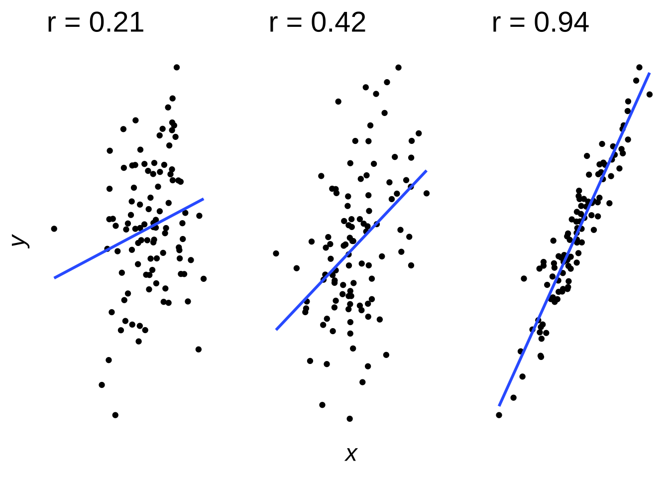
Figure 11.8: Weak, Moderate, and Strong Correlations

In the context of $t$-tests, effect sizes refer to differences. The effect size associated with a $t$-test is the difference between the observed mean statistic ($\bar{x}$ for a one-sample test, $\bar{d}$ for a repeated-measures test, or $\bar{x}_1-\bar{x}_2$ for an independent-groups test) and the population mean parameter ($\mu$ for a one-sample test, $\mu_d$ for a repeated-measures test, or $\mu_1-\mu_2$ for an independent-groups test) specified in the null hypothesis. However, because the size of an observed differences can vary widely depending on what is being measured and in what units, the raw effect size can be misleading to the point of uselessness. The much more commonly used measure of effect size for the difference between two things is the standardized effect size: the difference divided by the standard deviation of the data. The standardized effect size is actually so much more commonly used that when scientists speak of effect size for differences between two things, they mean the standardized effect size (the standardized is understood).

In frequentist statistics, the standardized effect size goes by the name of Cohen’s $d$. Cohen’s $d$ addresses the issue of the importance of sample size to statistical significance by removing $n$ from the $t$ equation, using standard deviations in the denominator instead of standard errors. Otherwise, the calculation of $d$ is closely aligned with the formulae for the $t$-statistics for each flavor of $t$-test. Just as each type of $t$-test is calculated differently but produces a $t$ that can be evaluated using the same $t$-distribution, the standardized effect size calculations for each $t$-test produces a $d$ that can be evaluated independently of the type of test.

For the one-sample $t$-test:

\[d=\frac{\bar{x}-\mu_{0}}{sd_{x}}\] for the repeated-measures $t$-test:

\[d=\frac{\bar{d}-\mu_d}{sd_{d}}\]

And for the independent-groups $t$-test:

\[d=\frac{\bar{x}_1-\bar{x}_2-\Delta}{sd_{p}}\] where the pooled standard deviation $sd_p$ is the square root of the pooled variance.

Note: although $d$ can take on an unbounded range of values, $d$ is usually reported as positive, so the $d$ we report is more accurately $|d|$.

The Cohen (2013)²⁰² guidelines for interpreting $d$ are:

Range of $d$	Effect-size Interpretation
$0.2 \le d < 0.5$	weak
$0.5 \le d < 0.8$	moderate
$d \ge 0.8$	strong

but, as Cohen himself wrote in the literal book on effect size:

“there is a certain risk inherent in offering conventional operational definitions for those terms for use in power analysis in as diverse a field of inquiry as behavioral science”

so please interpret effect-size statistics with caution.

11.3.0.1 Effect-size Examples

On this page, we have already calculated the values we need to produce $d$ statistics for examples of a one-sample $t$-test, a repeated-measures $t$-test, and an independent-groups $t$-test: all we need are the differences and the standard deviations from each set of calculations.

11.3.0.1.1 One-sample $d$ example

For our one-sample $t$-example, we had a set of temperatures produced by 10 freezers:

Freezer	Temperature ($^{\circ}C$)
1	-2.14
2	-0.80
3	-2.75
4	-2.58
5	-2.26
6	-2.46
7	-1.33
8	-2.85
9	-0.93
10	-2.01

The mean temperature is -2.01, and the standard deviation of the temperatures is 0.74. In this example, the null hypothesis was $\mu \ge 0^{\circ}C$, so the numerator of the $d$ statistic is $-2.01-0$, with the denominator equal to the observed standard deviation:

\[d=\frac{\bar{x}-\mu}{sd_x}=\frac{-2.01-0}{0.74}=-2.71\] For these data, $d=-2.71$, which we would report as $d=2.71$. Because $d\ge0.8$, these data represent a large effect.

11.3.0.1.2 Repeated-measures $d$ example

For our repeated-measures $t$-test example, we used the following data about ovens and cakes:

Cake	Pre-bake ($^{\circ} C$)	Post-bake ($^{\circ} C$)	Difference (Post $-$ Pre)
1	20.83	100.87	80.04
2	19.72	98.58	78.86
3	19.64	109.09	89.44
4	20.09	121.83	101.74
5	22.25	122.78	100.53
6	20.83	111.41	90.58
7	21.31	103.96	82.65
8	22.50	121.81	99.31
9	21.17	127.85	106.68
10	19.57	115.17	95.60

As when calculating the $t$-statistic, to calculate $d$ we are only interested in the difference scores. The mean difference score is 92.54 and the standard deviation of the difference scores is 9.77. We previously tested these data with both $H_0: \mu_d\le0^{\circ}C$ and $H_0: \mu_d\le90^{\circ}C$: let’s just examine the effect size for $H_0:\mu_d\le90^{\circ}C$ but keep in mind that effect size – like $t$’s and $p$-values – depends in part on the choice of null hypothesis. With $H_0: \mu_d=90$:

\[d=\frac{\bar{x}-\mu}{sd_x}=\frac{92.54-0}{9.77}=9.48\] The $d$ for these data is 9.48, indicating a large effect.²⁰³

11.3.0.1.3 Independent-groups $d$ Example

Finally, for the independent-groups $t$-test example, we examined the following data:

Time to Toast (s)
Mark I	Mark II
4.72	9.19
7.40	11.44
3.50	9.64
3.85	12.09
4.47	10.80
4.09	12.71
6.34	10.04
3.30	9.06
7.13	6.31
4.99	9.44

The numerator for $d$ for independent groups is the difference between the means $\bar{x}_1-\bar{x}_2$ and the hypothesized population-level difference $\mu_1-\mu_2$. For these data, the null hypothesis was $\mu_1-\mu_2=0$, so for this $d$, the numerator is simply $\bar{x}_1-\bar{x}_2=-5.09$. The denominator is the pooled standard deviation, which is the square root of the pooled variance; for these data, the pooled standard deviation is $=. Thus:

\[d=\frac{-5.09}{1.66}\] and $d=|d|=3.07$ represents a large effect.

11.3.0.2 A Note on Effect Size

The main difference between a $t$ statistic and its corresponding $d$ statistic is the sample size. That’s by design: effect size measurement is meant to remove the impact of sample size from assessing the magnitude of differences. Thus, it is possible to have things like statistically significant effects with very small ($< 0.2$) sizes. Another possible outcome of that separation is that the test statistic and the effect size statistic can be distinct to the point of disagreement: a small, medium, or even large $d$ value can be computed for data where there is no significant effect. If there is no significant effect, then there is no effect size to measure: please don’t report an effect size if the null hypothesis hasn’t been rejected.

11.4 Power of $t$-tests

11.4.0.1 What is power?

Figure 11.9: Not very helpful, Cersei

Statistical power is the rate at which population-level similarities (as in a correlation) or differences (as in a $t$-test) show up in a statistical test (which is, by definition, a sample-level test). As noted in Classical and Bayesian Inference, in the Classical (Frequentist) framework, there are two states of nature for a population-level effect – it either exists or does not – and two possibilities for the result of a statistical test – either reject $H_0$ or continue to assume $H_0$. Table 11.1 is a decision table outlining the possible outcomes of null hypothesis statistical testing.

Table 11.1: Classical Null Hypothesis Statistical Testing Decision Table
		Is a Population-level Effect Present?
		Yes	No
Decision Regarding $H_0$	Reject $H_0$	Hit	$\alpha$ error
Decision Regarding $H_0$	Continue to Assume $H_0$	$\beta$ Error	$H_0$ Assumption Correct

There are two types of errors we can make in this framework. The Type-I error, also known as the $\alpha$ error, is a false alarm: it happens when is no effect – similarity or difference – present in the population-level data but we reject $H_0$ regardless. The Type II error, also known as the $\beta$ error, is a miss: it happend when there is an effect – a similarity or a difference – present in the population-level data but we continue to assume $H_0$ regardless.

The rate at which we make the $\alpha$ error is more-or-less the $\alpha$ rate.²⁰⁴ When we set the $\alpha$ rate – most frequently it is set at $\alpha = 0.05$, but more stringent rates like $\alpha=0.01$ or $\alpha=0.001$ are also used – we are implicitly agreeing to a decision-making algorithm that will lead to false alarms $(100\times\alpha)$% of the time given the assumptions of the statistical test we are using.

For example, if we are conducting a one-sample $t$-test with $H_0: \mu = 0$, $H_1: \mu \ne 0$, $df=20$, and $\alpha=0.05$, we are saying that our null hypothesis is that our observed sample is drawn from a normal distribution with $\mu=0$. If the mean of the population from which we are sampling is, in fact, 0, and we were to run the same experiment some large, infinity-approaching number of times, we would expect the resulting $t$-statistics to be distributed thus:

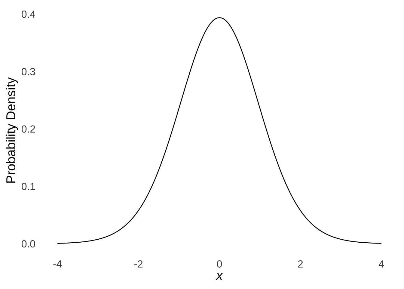
Figure 11.10: A Basic $t$-distribution with $df=20$

With $\alpha=0.05$ and a two-tailed test, the rejection regions for the $t$-distribution with $df=20$ are defined as anything less than $t=-2.09$ and anything greater than $t=2.09$. If an observed $t$ is located in either of those regions, $H_0$ will be rejected. However, if the null hypothesis is true, then exactly 5% of $t$-statistics calculated based on draws of $n=21$ (that’s $df+1$) from a normal distribution with a mean of 0 will naturally live in those rejection regions, as we can see by superimposing line segments representing the boundaries of the rejection regions over the null $t$-distribution in Figure 11.11:

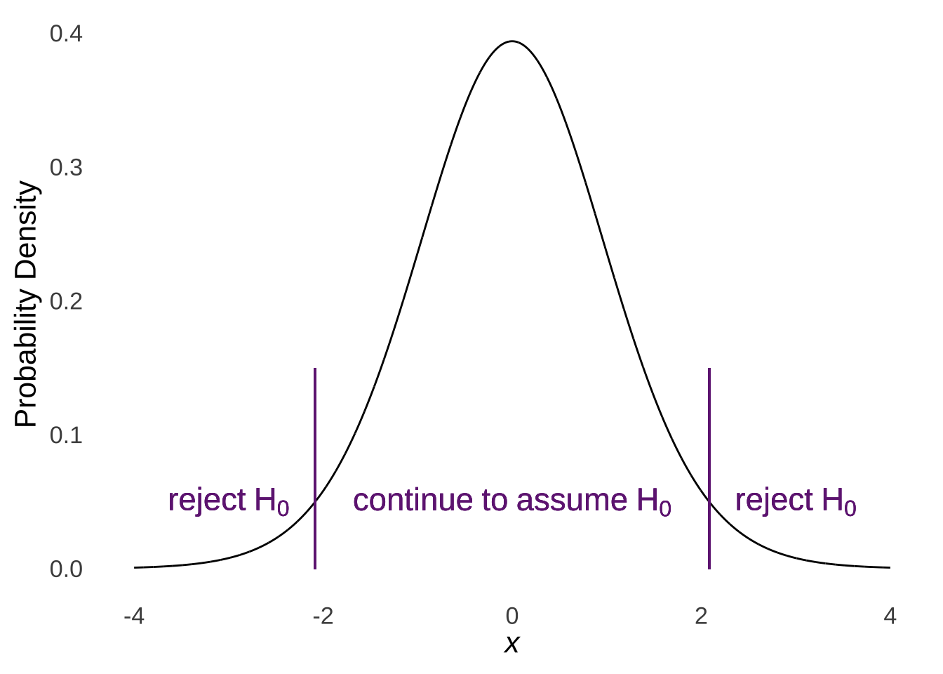
Figure 11.11: Rejection Regions for a Basic $t$-distribution with $df=20$

We can simulate the process of taking a large number of samples from a normal distribution with $\mu=0$ with the rnorm() command in R. In addition to $\mu=0$, we can stipulate any value for $\sigma^2$ because it will all cancel out with the calculation of the $t$-statistic. Let’s take 1,000,000 samples of $n=21$ each from a normal distribution with $\mu=0,~\sigma^2=1$ and calculate a one-sample $t$-statistic for each based on $H_0:~\mu=0$ ($t=\frac{\bar{x}}{s/\sqrt{n}}$). With $df=n-1=20$, the $t$-values that define a lower-tail area of 2.5% and an upper-tail area of 2.5% are -2.09 and 2.09, respectively. Taking repeated samples from the normal distribution defined by the null hypothesis, we should expect 2.5% of the observed samples to produce $t$-statistics that are less than or equal to -2.09 and another 2.5% to produce $t$-statistics that are greater than or equal to 2.09. If we take 1,000,000 samples, that means about 25,000 should be less than or equal to -2.09 and another 25,000ish should be greater than or equal to 2.09. Let’s see what we get!

n=21 #Number of observations per sample
k=1000000 #Number of samples
t.statistics<-rep(NA, k) #Vector to hold the t-statistics

for (i in 1:k){
  sample<-rnorm(n, mean=0, sd=1)
  t<-mean(sample)/
    (sd(sample)/sqrt(n))
  t.statistics[i]<-t
}

t.table<-cut(t.statistics, c(-Inf, qt(0.025, df=20), qt(0.975, df=20), Inf))
table(t.table)

## t.table
## (-Inf,-2.09] (-2.09,2.09]  (2.09, Inf] 
##        24907       950070        25023

That is all to say that the rates at which $\alpha$-errors are made are basically fixed by the $\alpha$-rate.

The rates at which $\beta$-errors are made are not fixed, and are only partly associated with $\alpha$-rates. In the example illustrated in Figure 11.11, any observed $t$-statistic that falls between the rejection regions will lead to continued assumption of $H_0$. That would be true even if the sample were drawn from a different distribution than the one specified in the null, that is, if the null were false. That is the $\beta$ error: when the null is false – as in, the sample comes from a different population than the one specified in the null – but we continue to assume $H_0$ anyway. The complement of the $\beta$ error – the rate at which the the null is false and $H_0$ is rejected in favor of $H_1$ – is therefore $1-\beta$.

Power is the complement of the $1-\beta$: the complement of the $\beta$-rate.

Power is the rate at which the null hypothesis is rejected given that the alternative is true.

To illustrate, please imagine that $H_0$ defines a null model with $\mu=3$ and $\sigma^2=1$, but that the observed samples instead come from a different distribution – an alternative distribution – with $\mu=4$ and $\sigma^2=1$. Figure 11.12 presents both the null and alternative parent distributions (i.e., the normals).

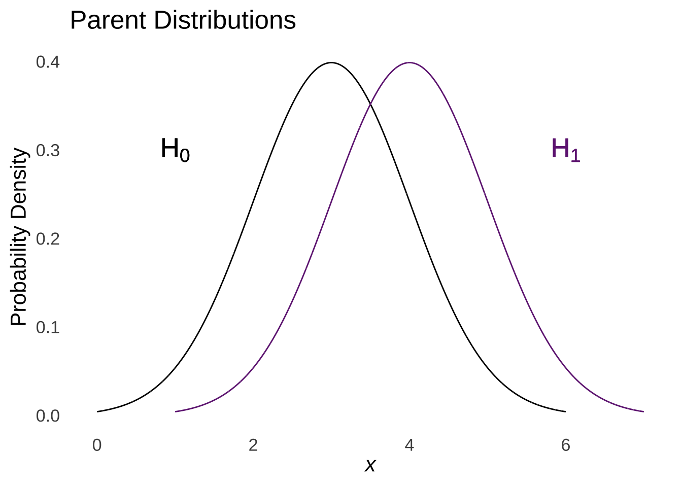
Figure 11.12: Null and Alternative Parent Distributions

If this were the case, the central limit theorem tells us that the sample means from the null model will be (approximately) normally distributed with a mean equal to the mean of the null model and a variance equal to the variance of the null model divided by $n$ – $\bar{x}_0 \sim N(\mu_0, \sigma+0^2/n)$ – and the sample means from the alternative model will be (approximately) normally distributed with a mean equal to the mean of the alternative model and a variance equal to the variance of the alternative model divided by $n$ – $\bar{x}_1 \sim N(\mu_1, \sigma_1^2/n)$, as shown in Figure 11.13:

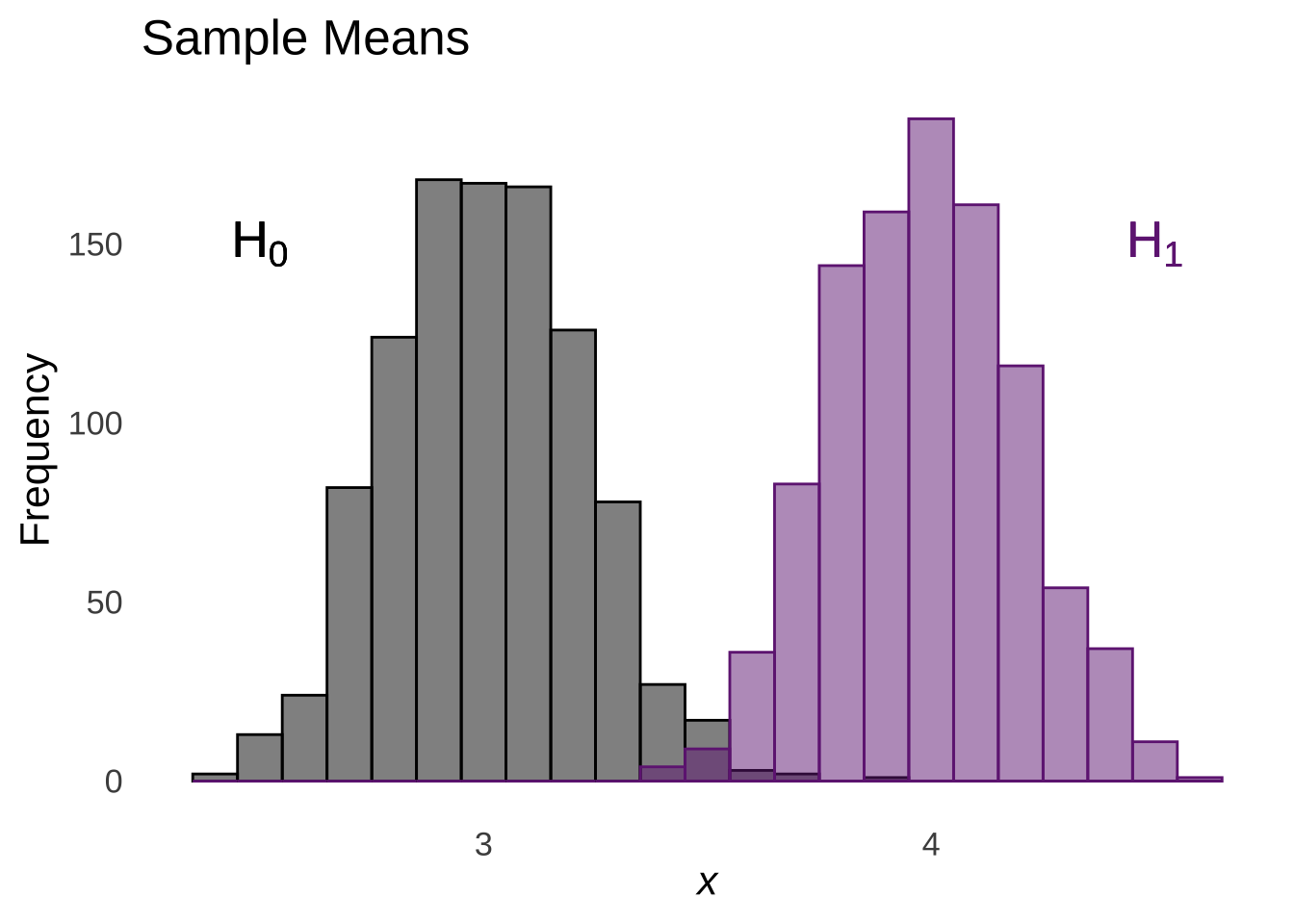
Figure 11.13: Sample Means Drawn from Null Model (left) and Alternative Model (right)

These two distributions of sample means – the one sampled from the null model and the one sampled from the alternative model – are basically identical except the one from the alternative is shifted one unit to the right.

Each of the samples may represent the results of an experiment: a set of $22$ observations; some observed in a world where the population mean $(\mu)$ is equal to $3$; the others observed in a world where $\mu=4$. We can add inferential statistics to the example by imagining that these are results of a hypothetical experiment with a one-tailed hypothesis:

\[H_0: \mu\le3\]

\[H_1=\mu>3\] \[df=21\]

\[\alpha = 0.05\]

Given the specifications of our experiment, we can calculate a critical $t$-value by finding the value of the $t$ distribution with $df=21$ that puts $\alpha=0.05$ in the upper tail (upper because this is a one-tailed test with $H_1$ in the positive direction):

\[t_{crit}^{\alpha = 0.05}(21) = 1.72\] Thus, we know that any $t_{obs} > 1.72$ – regardless of whether it is sampled from the null or from the alternative distribution – will lead to rejecting $H_0$.

Figure 11.14 demonstrates the steps of calculating the $t$-statistics asssociated with each of the samples drawn for this example. The top chart of Figure 11.14 shows the $t$ numerator for each sample – each observed sample mean $\bar{x}$ minus the null-hypothesis mean $\mu = 3$. The $t$-numerators for the samples drawn from the alternative distribution generally live to the right of the samples drawn from the null distribution. The middle chart of Figure 11.14 shows the distribution of standard errors for the samples: standard deviation of the observations in each sample divided by the square root of the number of observations in those samples $(sd\sqrt{n})$. Note that since sample variances are distributed as $\chi^2$ distributions, and the standard error of a sample is the square root of a sample variance divided by $n$, the distribution of standard errors will be all-positive and skewed positively (with the degree of the skew dependent on the $df$ and smaller than the skew of the corresponding sample variances because of the square-root operation). The key thing for now is that the distributions of standard errors from each set of samples is going to be about the same; we can see by overlaying the histograms of standard errors in the example data that they are virtually identical.

Finally, the distributions of $t$-statistics – the numerators described above divided by the denominators described above – are shown in the bottom chart of Figure 11.14, along with a vertical line indicating the critical value $t = 1.72$.

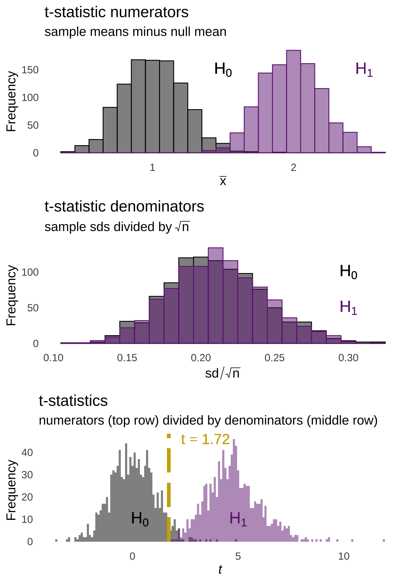
Figure 11.14: Steps of Calculating $t$-statistics for Samples Drawn from Null and Alternative Distributions

The observed results for the example data are shown in Table 11.2, which is an update of Table 11.1 with the results of the simulation from this section. It is (I hope) instructive to see that for the 1,000 samples taken for which the null hypothesis was true (note: you can only say things like “the null hypothesis was true” for simulations, we definitely can’t say that for results from an experiment), about 5% of the samples result in type-I errors which is what we expect when $\alpha = 0.05$. However, what’s more important for this section of the book is what happens for the 1,000 samples that were generated from the alternative distribution. In all of those cases, the null hypothesis was false (again, a thing you can only say in simulations). Some of the samples ended up in continuing to assume the null hypothesis because $t_{obs}<t_{crit}$, or, equivalently, $p > \alpha$: those are type-II errors. Other samples – in this case, the majority of the samples – resulted in rejecting $H_0$: those are the correct rejections, the proportion of times that happens in the long run is the power.

Table 11.2: Decision Table for the Example Data
		Is a Population-level Effect Present?
		Yes: 1,000 samples	No: 1,000 samples
Decision Regarding $H_0$	Reject $H_0$	999 (99.9%) correct rejections	49 (4.9% ) $\alpha$ error
Decision Regarding $H_0$	Continue to Assume $H_0$	1 (0.1% ) $\beta$ Error	951 (95.1% ) $H_0$ Assumption Correct

The minimum limit to power, given the stipulated $\alpha$-rate, is $\alpha$ itself. That minimum would occur if the alternative hypothesis completely overlapped the null distribution: the only place from which a sample could be drawn that would lead to rejecting $H_0$ would be in the rejection region. Of course, an alternative distribution can’t be identical to the null distribution – otherwise it wouldn’t really be an alternative to the null – so the case of complete overlap is really a theoretical, asymptotic limit. The maximum limit to power is $1$, occurring if there were no overlap whatsoever between the null and alternative distributions. That situation is also theoretically impossible in the case of the $t$-test because $t$-distributions, like normal distributions, extend forever in each direction, but given enough separation between null and alternative distributions, the power can approach $1$. Figure 11.15 illustrates both upper limits in the context of a one-tailed test (just for the graphical simplicity afforded by a single-tailed rejection region.)

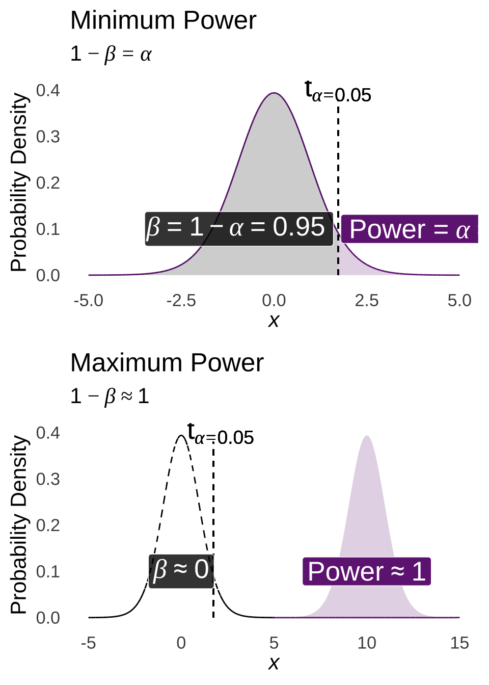
$Minimum Power ($\alpha$ and Maximum Power ($\approx 1$)$

Figure 11.15: Minimum Power ($\alpha$ and Maximum Power ($\approx 1$)

$Settle down, Palpatine. Power has a lower limit of $\alpha$ and an upper limit of 1.$

Figure 11.16: Settle down, Palpatine. Power has a lower limit of $\alpha$ and an upper limit of 1.

11.4.0.2 Power Analysis for $t$-tests

In the foregoing description of power, certain values were stipulated in order to estimate power. Power analysis is a procedure for using stipulations on effect size and power to predict required sample size, stipulating effect size and sample size to predict power, and/or stipulating power and sample size to predict effect size. Typically, power analyses stipulate the first pair: given a desired power level – 0.8 and 0.9 are popular choices – and an effect size – which is predicated on the approximate effect size expected, usually based on the results of previous similar experiments – to estimate the number of participants that will be required in an experiment. Such analyses are particularly valuable to planning experiments and/or securing research funding: if one is planning a study or asking a funding agency for resources, one would like to be able to show a relatively high probability of finding significant effects (given that population-level effects exist).

When working with uncommon analyses (e.g., a complex multiple regression model) and/or variables with unknown distributions (e.g., an index variable created for the purposes of a single novel experiment), a simulation like the one in this section would be exactly how one would estimate power: simulate lots of data, calculate inferential statistics, and report a proportion of significant effects as an estimate of long-run expectations. $t$-tests, though, are pretty common, and we know lots about how sample means, standard errors, and $t$-statistics are distributed. Samples from null distributions produce $t$-statistics from a regular-ass $t$-distribution with $df = n-1$; differences of sample means produce $t$-statistics from a regular-ass $t$-distribution with $df = n_1 - n_2 -2$. Samples from alternative distributions also produce $t$-statistics, but they’re not distributed like a regular-ass $t$. The expectation of $t$-statistics from distributions that are not the null is known as the noncentral $t$-distribution.

11.4.0.2.1 The Noncentral $t$-distribution

You may have noticed that the distribution of $t$-statistics for samples from the alternative distribution shown in Figure 11.14 is a little stretched and skewed away from 0 (if you didn’t, please feel free to go back and look again). You may also remember that the distributions $t$ numerators for samples from the alternative were shifted away from 0. You may further remember that the distributions of standard errors for the two sets of samples were pretty much identical and that both had a slight positive skew. The relationship between the numerators and the denominators of $t$-statistics for data sampled where the null is false gives the noncentral $t$-distribution its shape.

When sampling from an alternative distribution, some of the samples are going to have means are going to be very far away from the null mean and also have standard errors that are relatively small (and because of the expected distribution of standard errors, there tend to be more small standard errors than big ones): cases like that are what gives the distribution of $t$-statistics for alternative-model samples a bit of skew. In situations like that of the simulated example above, the alternative distribution is positively shifted from the null model so that skew is positive; when the alternative model is negatively shifted away from the null model, the skew of $t$-statistics for the samples from the alternative model will be negatively skewed. That skew doesn’t happen for samples from the null model because large $t$-statistics are balanced between values greater than the mean and less than the mean; that balance doesn’t happen for the alternative samples because the whole alternative distribution is shifted.

The noncentral $t$-distribution has two sufficient statistics, both related to the process of calculating $t$-statistics. The first is $df$; that is simply $df=n-1$ for single samples or samples of differences or $df=n_1+n_2-2$ for differences of sample means. The second is the noncentrality parameter $\delta$:

\[\delta=\frac{\mu_0-\mu}{\sigma/\sqrt{n}}\] where $\mu_0$ is the null mean, $\mu$ is the alternative mean, $\sigma$ is the standard deviation of the alternative distribution (and of the null distribution; those are always the same), and $n$ is the number of observations. The noncentrality parameter is closely related to Cohen’s $d$. When we calculate $d$, the numerator is the difference between the observed value ($\bar{x}$, $\bar{d}$, or $\bar{x}_1-\bar{x}_2$) and the population mean value of the null model ($\mu_0$, $\mu_d$, or $\mu_1-\mu_2$). In power analysis, we stipulate a value for the alternative mean; that becomes the $\mu$ for the numerator of the noncentrality parameter $\delta$. From there, all we have to do is multiply the intended effect size for an experiment by $\sqrt{n}$ to get $\delta$.

Figure @ref:(fig:noncentralt) depicts different noncentral $t$ curves for different values of $df$ when $\delta = 1$ (top) and different noncentral $t$ curves for different values of $\delta$ when $df = 30$.

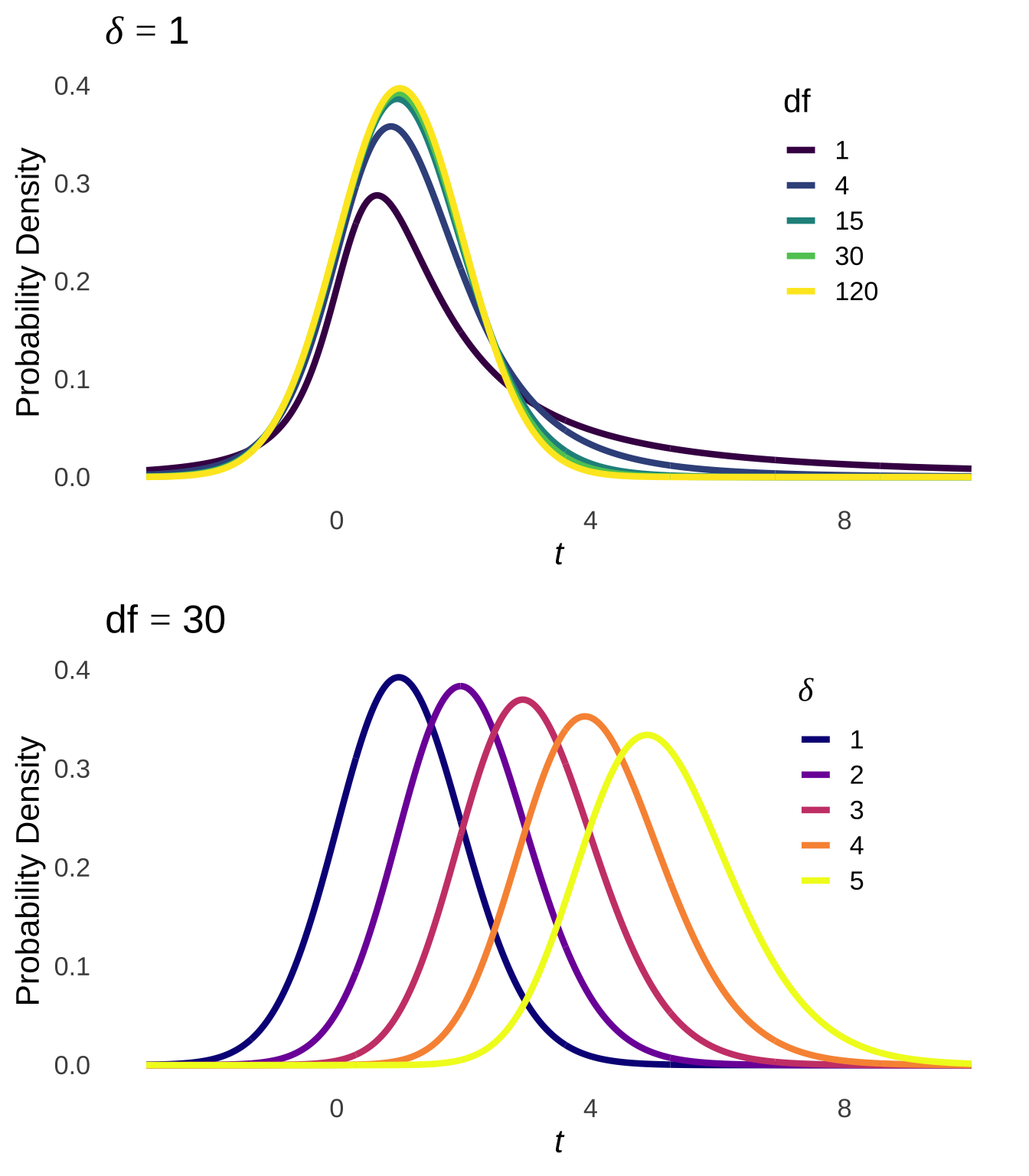
$Noncentral $t$-distribution Curves with Constant $\delta$ and Varying $df$ (top) and with Constant $df$ and Varying $\delta$ (bottom)$

Figure 11.17: Noncentral $t$-distribution Curves with Constant $\delta$ and Varying $df$ (top) and with Constant $df$ and Varying $\delta$ (bottom)

Power analyses for $t$-tests can be conducted by solving simultaneous equations: given a null distribution with rejection regions defined by $\alpha$ and the effect size $d$, we can calculate the area under the noncentral $t$ curve that is in the rejection regions – the power – as a function of $n$. If you’d rather not – and I wouldn’t blame you one bit – there are several software packages that can give convenient power analyses with a minimum effort. For example, using the pwr package, we can use the following code to find out how many participants we would expect to need to have power of 0.8 given an effect size $d=0.5$ (for a medium-sized effect) and an $\alpha$-rate of 0.05 for a two-tailed hypothesis on a one-sample $t$-test:

library(pwr)
pwr.t.test(n=NULL, d=0.5, sig.level=0.05, power=0.8, type="one.sample", alternative="two.sided")

## 
##      One-sample t test power calculation 
## 
##               n = 33.36713
##               d = 0.5
##       sig.level = 0.05
##           power = 0.8
##     alternative = two.sided

Using the same pwr package, we can also plot a power curve indicating the relationship between $n$ and power by wrapping the pwr.t.test() command in plot():

plot(pwr.t.test(n=NULL, d=0.5, sig.level=0.05, power=0.8, type="one.sample", alternative="two.sided"))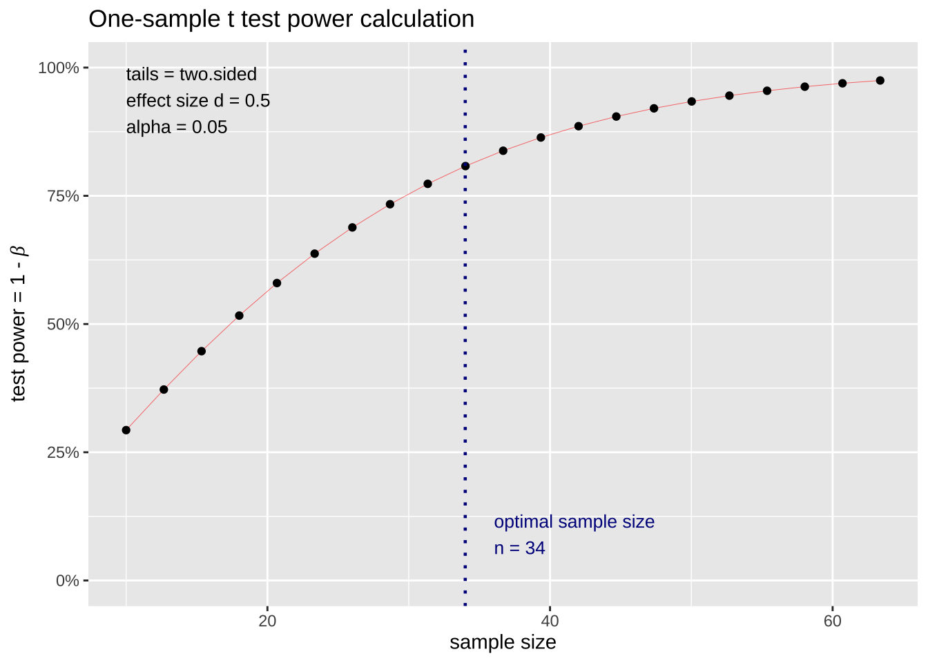

11.4.0.3 Notes on Power

11.4.0.3.1 “Observed” or “Retrospective” Power

Occasionally, a scientific paper will report the “observed” or “retrospective” power of an experiment that has been conducted. That means that based on the observed difference between a sample mean (or a mean difference, or a difference of sample means) and the null hypothesis $\mu$, the variance (or pooled variance) of the data, the $\alpha$-rate, and $n$, the authors have calculated what the power should have been, assuming that an alternative distribution can be estimated from the observed data. That is a bad practice, for at least a couple of reasons. First: it assumes that the alternative distribution is something that can be estimated rather than stipulated, putting aside that the point of power analysis is to stipulate various reasonable conditions for an experiment. Second: citing the probability of an event after an event has occurred isn’t terribly meaningful – it’s like losing a bet but afterwards saying that you should have won because you had a 51% chance of winning. So, like reporting an effect size for a non-significant effect: don’t do it.

11.4.0.3.2 Misses vs. True Null Effects

In the null-hypothesis testing framework, failing to reject the null hypothesis can happen for one of two reasons:

There is a population-level effect but the scientific algorithm didn’t detect it, in other words: a type-II error
There is no population-level effect, in other words: a correct continuation of assuming $H_0$.

A major flaw of frequentist null-hypothesis testing is that there is no way of knowing whether reason 1 (a type-II error) or reason 2 (a correct assumption of $H_0$ has occurred) is behind a failure to reject the null. If there actually is no population-level effect, a non-significant statistical result could either be the result of a failed experiment or a successful experiment: there’s no way of knowing.

Thus, there is perfectly-warranted skepticism regarding null results: statistical analyses that show neither differences nor similarities, which in the null-hypothesis testing framework take the form of failure to reject $H_0$. Such results go unsubmitted and unpublished at rates that we can’t possibly know precisely because they are neither submitted nor published (this is known as the file-drawer effect). The problem is that sometimes null results are really important. A famous example is the finding that the speed of light is unaffected by the rotation of the earth. In psychological science, null results in cognitive testing between people of different racial, ethnic, and/or gender identification are both scientifically and socially important; if we only publish the relative few studies that find small differences (which themselves may be type-I errors), those findings receive inordinate attention among what should be a sea of contradictory findings.

In classical statistics, confidence intervals likely provide the best way of the available options to support null results – confidence intervals that include 0 imply that 0 will be sampled in the majority of repeated tests. Bayesian methods include more natural and effective ways of producing support for the null: in the Bayesian framework, results including zero-points can be treated as would be any other posterior distribution. One can create Bayesian credible interval estimates that include values like 0 and can calculate Bayes Factors indicating support for posterior models that include null results. So: point for Bayesians there.

11.5 Bayesian $t$-tests

We previously used Bayesian methods to create a posterior distribution on a proportion parameter $\pi$ using the Metropolis-Hastings algorithm. From that distribution, we could calculate things like the probability that the parameter fell into a given range, or the highest-density interval of the parameter.

We can do the same thing for mean data. For a relatively (that word is doing a lot of work here) simple example, we can use the MH algorithm to produce a posterior distribution on the mean freezer temperature from the one-sample $t$-test example above. (Note: this code also calculates the posterior distribution on the variance, but I included that more as a way to let the variance…vary).

#MCMC estimation of one-sample data (the freezer data)
iterations<-1000000
means<-c(-2, rep(NA, iterations-1))
vars<-c(0.5, rep(NA, iterations-1))

for (i in 2:iterations){
  mean.prop<-runif(1,-5, 1)
  vars.prop<-runif(1, 0.00001, 2)
  u<-runif(1)
  r<-prod(dnorm(freezer.data, mean.prop, sqrt(vars.prop)))/
    prod(dnorm(freezer.data, means[i-1], sqrt(vars[i-1])))
  if (r>=1){
    means[i]<-mean.prop
    vars[i]<-vars.prop
  } else if (r > u){
    means[i]<-mean.prop
    vars[i]<-vars.prop
  } else {
    means[i]<-means[i-1]
    vars[i]<-vars[i-1]
  }
}

ggplot(data.frame(means), aes(means))+
  geom_histogram(binwidth=0.02)+
  theme_tufte(base_size=16, base_family="sans", ticks=FALSE)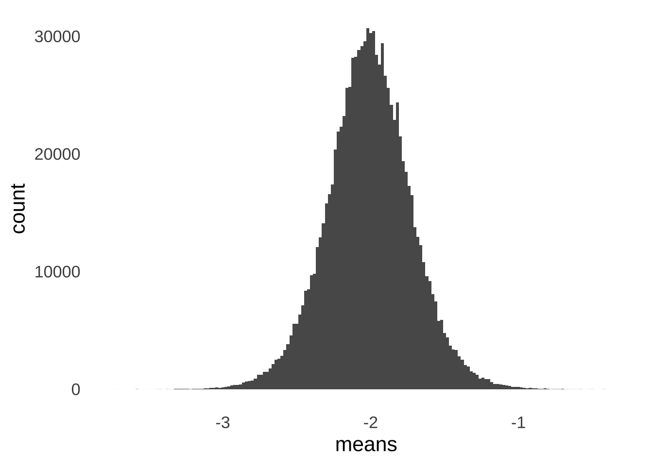

Figure 11.18: Posterior Distribution of Mean Freezer Temperatures

This posterior distribution indicates that the probability that the mean freezer temperature is less than 0 is 1, and that the 95% highest-density interval of the mean is $p(-2.59 \le \bar{x} \le -1.44)=0.95$ .

But, Bayesian analyses requiring more complexity can be a problem, especially if we are interested in calculating the Bayes factor. When we calculated the Bayes factor comparing two binomial models that differed only in the specification of the $\pi$ parameter, the change from the prior odds to the posterior odds was given by the ratio of two binomial likelihood formulae:

\[B.F.=\frac{p(D|H_1)}{p(D|H_2)}=\frac{\frac{20!}{16!4!}(0.8)^{16}(0.2)^4}{\frac{20!}{16!4!}(0.5)^{16}(0.5)^4}=\frac{(0.8)^{16}(0.2)^4}{(0.5^{16}(0.5)^4)}\] For more complex models than the binomial – even the normal distribution works out to be a much more complex model than the binomial model – the Bayes factor is calculated by integrating competing models over pre-defined parameter spaces, that is, areas where we might reasonably expect the posterior parameters to be. Given a comparison between a model 1 and a model 0, that looks basically like this:

\[B.F._{10}=\frac{\int p(D|\theta_{H_1})p(\theta_{H_1})d\theta_{H_1}}{\int p(D|\theta_{H_0})p(\theta_{H_0})d\theta_{H_0}}\] where $\theta$ represents the model parameter(s). In addition to the difficulty of integrating probability distributions, specifying the proper parameter space involves its own set of tricky decisions.

Several R packages have recently been developed to make that process much, much easier. In this section, I would like to highlight the BayesFactor package²⁰⁵, which does a phenomenal job of putting complex Bayesian analyses into familiar and easy-to-use formats.

ttestBF() is a key function in the BayesFactor package. It produces results of Bayesian $t$-tests using commands that are nearly identical to those used in R to produce results of classical $t$-tests. Before we get to those blessedly familiar-looking commands, let’s take a brief look at the theory behind the Bayesian $t$-test.

The key insight that makes the Bayesian $t$-test both computationally tractable and more familiar to users of the classical version comes from Gönen et al (2005), who formulated $t$-test data in a way similar to the regression-model form of the $t$-test. Taking for example an independent-groups $t$-test, the observed data points $y$ in each group are distributed as normals with a mean determined by the grand mean of all the data $\mu$ plus or minus half the (unstandardized) effect size $\delta$ and a variance equal to the variance of the data:

\[Group~1:~y_{1i}\sim N \left(\mu+\frac{\sigma \delta}{2}, \sigma^2 \right)\] \[Group~2:~y_{2j}\sim N \left(\mu-\frac{\sigma \delta}{2}, \sigma^2 \right)\] where $i=1, 2, ...n_1$ and $j=1, 2, ... n_2$.

This insight means that the null model (not to be confused with a null hypothesis because that’s the other kind of stats – this is just a model that says there is no difference between the groups) $M_0$ is one where there is no effect size ($\delta=0$), and that can be compared to another model $M_1$ where there is an effect size ($\delta\ne0$). Moreover, a prior distribution can be stipulated for $\delta$ and, based on the data, a posterior distribution can be derived based on that prior distribution and the likelihood of the data given the prior.²⁰⁶

For the prior distribution, the Cauchy distribution – also awesomely known as The Witch of Agnesi – is considered ideal for its shape and its flexibility. The Cauchy distribution has a location parameter ($x_0$) and a scale parameter (formally $\gamma$ but the BayesFactor output calls it r so we’ll comply with that), but for our purposes the location parameter will be fixed at 0. When the scale parameter $r=1$, the resulting Cauchy distribution is the $t$-distribution with $df=1$. The ttestBF() command in the BayesFactor package allows any positive value for $r$ to be entered in the options: smaller values indicate prior probabilities that favor smaller effect sizes; larger values indicate prior probabilities favoring larger effect sizes. Figure 11.19 illustrates the Cauchy distribution with the three categorical options for width of the prior distribution in the ttestBF() command: the default “medium” which corresponds to $r=1/\sqrt{2}\approx 0.71$, “wide” which corresponds to $r=1$, and “ultrawide” which corresponds to $r=\sqrt{2}\approx 1.41$.

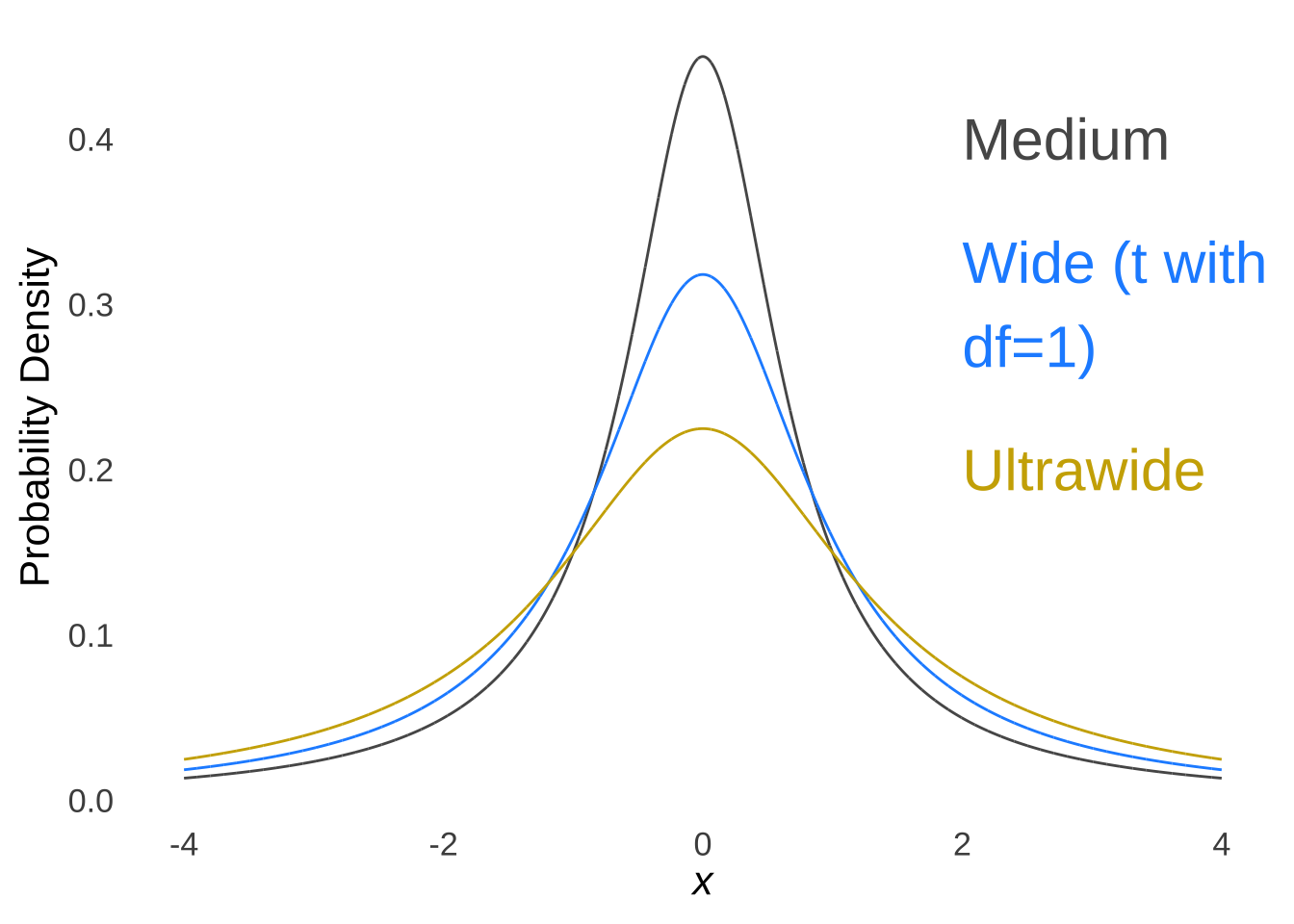
$The Cauchy Distribution with Scale Parameters $\frac{1}{\sqrt{2}}$ (for Medium Priors), $1$ (for Wide Priors), and $\sqrt{2}$ (for Ultra-Wide Priors)$

Figure 11.19: The Cauchy Distribution with Scale Parameters $\frac{1}{\sqrt{2}}$ (for Medium Priors), $1$ (for Wide Priors), and $\sqrt{2}$ (for Ultra-Wide Priors)

The main output of the ttestBF() command is the Bayes factor between model 1 – the model determined by the maximum combination of the prior hypothesis and likelihood function – and model 2 – the model that assumes no effect size. To interpret Bayes factors, the following sets of guidelines have been proposed – both are good – reposted here from the page on classical and Bayesian inference:

Jeffreys (1961)		Kass & Raftery (1995)
Bayes Factor	Interpretation	Bayes Factor	Interpretation
$1 \to 3.2$	Barely Worth Mentioning	$1 \to 3.2$	Not Worth More Than a Bare Mention
$3.2 \to 10$	Substantial	$3.2 \to 10$	Substantial
$10 \to 31.6$	Strong	$10 \to 100$	Strong
$31.6 \to 100$	Very Strong	$ $	Decisive
$ $	Decisive

The ttestBF() output also includes the value of $r$ that was used to define the Cauchy distribution for the prior and a margin-of-error estimate for the Bayes factor calculation (which will be ~0 unless there are very few data points in the analysis).

To start, let’s conduct a Bayesian $t$-test on the example data we used for the one-sample $t$-test:

library(BayesFactor)
ttestBF(c(freezer.data))

## Bayes factor analysis
## --------------
## [1] Alt., r=0.707 : 1701.953 ±0%
## 
## Against denominator:
##   Null, mu = 0 
## ---
## Bayes factor type: BFoneSample, JZS

The result of the Bayes factor analysis, which uses a Cauchy prior on $\delta$ with a scale parameter of $r=\frac{1}{\sqrt{2}}$ (which is the default for ttestBf() and the value one would use if expecting a medium-sized effect), indicates that the posterior odds in favor of the alternative model increase the prior odds by a factor of 1,702; that is, the posterior model is about 1,702 times as likely as the null model. That result agrees with the significant difference from 0 we got with the frequentist $t$-test – the alternative is more likely than the null.

We can also wrap the ttestBF() results in the posterior() command – specifying in the options the number of MCMC iterations we want to use – to produce posterior estimates of the population mean, the population variance, the effect size (delta), and a parameter called g that you do not need to worry about. To get summary statistics for those variables, we then wrap posterior() in the summary() command. While the Bayes factor is probably the most important output, the summary statistics on the posterior distributions help fill out the reporting of our results.

summary(posterior(ttestBF(freezer.data), iterations=5000))

## 
## Iterations = 1:5000
## Thinning interval = 1 
## Number of chains = 1 
## Sample size per chain = 5000 
## 
## 1. Empirical mean and standard deviation for each variable,
##    plus standard error of the mean:
## 
##          Mean       SD Naive SE Time-series SE
## mu    -1.9394   0.2914 0.004121       0.004665
## sig2   0.8064   0.5421 0.007666       0.009875
## delta -2.4195   0.7218 0.010208       0.013575
## g     30.3074 302.0684 4.271892       4.271892
## 
## 2. Quantiles for each variable:
## 
##          2.5%     25%     50%     75%   97.5%
## mu    -2.4986 -2.1222 -1.9453 -1.7703  -1.338
## sig2   0.2799  0.4742  0.6644  0.9713   2.163
## delta -3.9076 -2.9091 -2.4013 -1.9149  -1.091
## g      0.5149  2.0250  4.4691 11.7740 136.392

If we desire visualizations of the posterior distributions, we can wrap the posterior() command with plot() instead of summary (the traces indicate the different values of statistics produced at each iteration of the MCMC process).

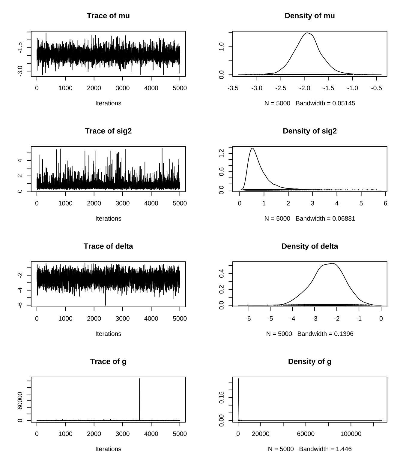
plot(posterior(ttestBF(freezer.data), iterations=5000))

As shown with the examples above, ttestBF() uses the same syntax as t.test(). It is therefore straightforward to translate the commands for the classical repeated-measures $t$-test into the Bayesian repeated-measures $t$-test (with the posterior() options in there for completeness)

ttestBF(prebake, postbake, paired=TRUE, mu=90)

## Bayes factor analysis
## --------------
## [1] Alt., r=0.707 : 5013899047 ±0%
## 
## Against denominator:
##   Null, mu = 90 
## ---
## Bayes factor type: BFoneSample, JZS

summary(posterior(ttestBF(prebake, postbake, paired=TRUE, mu=90), iterations=5000))

## 
## Iterations = 1:5000
## Thinning interval = 1 
## Number of chains = 1 
## Sample size per chain = 5000 
## 
## 1. Empirical mean and standard deviation for each variable,
##    plus standard error of the mean:
## 
##          Mean       SD Naive SE Time-series SE
## mu    -92.231    3.813  0.05393        0.05393
## sig2  142.048   95.780  1.35454        1.79205
## delta  -8.625    2.185  0.03090        0.04033
## g     261.477 1343.846 19.00485       19.00485
## 
## 2. Quantiles for each variable:
## 
##          2.5%    25%     50%     75%    97.5%
## mu    -99.495 -94.61 -92.269 -89.992  -84.298
## sig2   50.306  84.71 116.402 167.969  376.581
## delta -13.088 -10.07  -8.537  -7.103   -4.643
## g       6.299  24.00  53.255 142.063 1707.475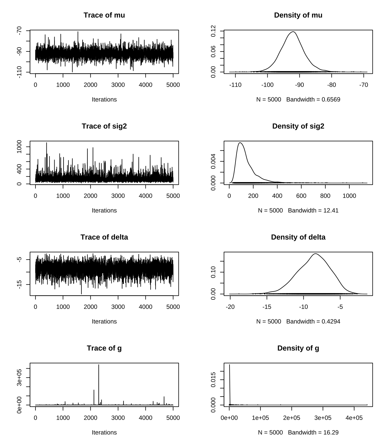

plot(posterior(ttestBF(prebake, postbake, paired=TRUE, mu=90), iterations=5000))

And it is just as easy to translate the independent-groups $t$-test into the Bayesian independent-groups $t$-test.

ind.groups.BF<-ttestBF(Mark.I, Mark.II, paired=FALSE)

ind.groups.BF

## Bayes factor analysis
## --------------
## [1] Alt., r=0.707 : 5682.522 ±0%
## 
## Against denominator:
##   Null, mu1-mu2 = 0 
## ---
## Bayes factor type: BFindepSample, JZS

summary(posterior(ind.groups.BF, iterations=5000))

## 
## Iterations = 1:5000
## Thinning interval = 1 
## Number of chains = 1 
## Sample size per chain = 5000 
## 
## 1. Empirical mean and standard deviation for each variable,
##    plus standard error of the mean:
## 
##                 Mean        SD  Naive SE Time-series SE
## mu             7.525    0.4140  0.005855       0.005855
## beta (x - y)  -4.823    0.8450  0.011951       0.013697
## sig2           3.335    1.2831  0.018145       0.022144
## delta         -2.778    0.6918  0.009784       0.012387
## g            102.315 5150.4955 72.839005      72.839005
## 
## 2. Quantiles for each variable:
## 
##                 2.5%    25%    50%    75%   97.5%
## mu            6.7260  7.258  7.522  7.793   8.338
## beta (x - y) -6.4260 -5.377 -4.841 -4.296  -3.118
## sig2          1.6297  2.441  3.071  3.923   6.621
## delta        -4.1232 -3.246 -2.763 -2.315  -1.435
## g             0.7811  2.696  5.658 13.585 155.222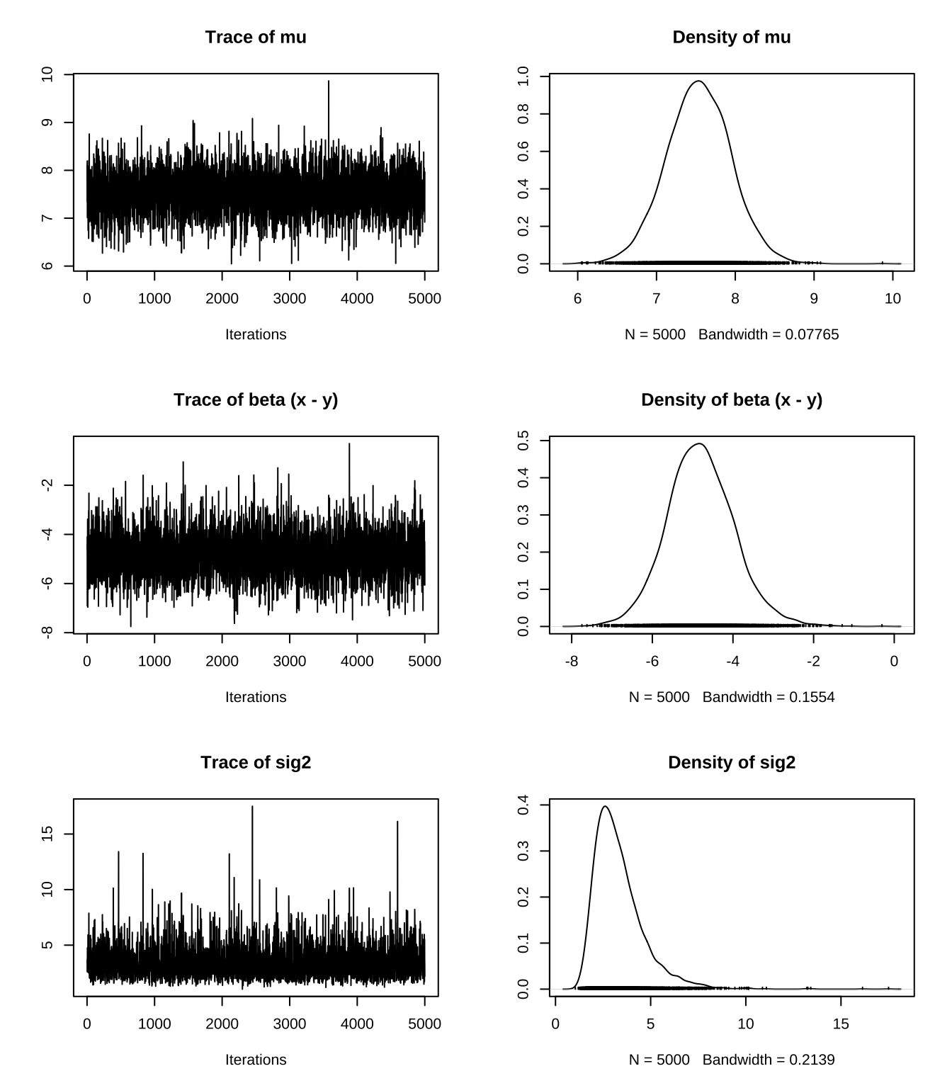

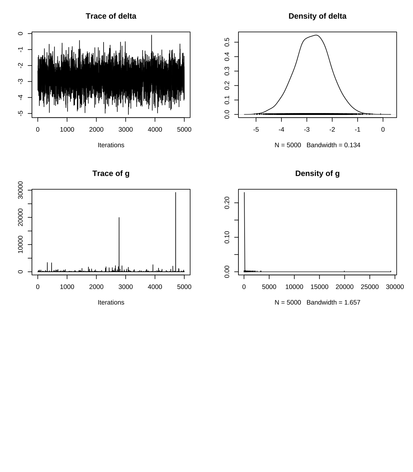
plot(posterior(ind.groups.BF, iterations=5000))

I think it would be more appropriate to say that the limit of the variance of the sample means as $n$ goes to infinity is $0$ and that the proper mathematical way to say it is not $\sigma^2/\infty=0$ but rather \[\lim_{n \to \infty}\frac{\sigma^2}{n}=0\] but I’m not much of a math guy.↩︎
The qualifier “finite” is used to exclude a sample of the entire population, because in that (practically impossible) case the only possible sample mean is the population mean↩︎
I know, I glanced over the links above and $0^{\circ}C$ is not cold enough. Let’s just go with it for the example↩︎
Don’t delete your raw data, though! We won’t need them for the rest of the calculations, but that doesn’t mean they might not come in handy for a different analysis.↩︎
Although if there is unequal $n$ between the two groups, it is more likely that the data violate the homoscedasticity assumption ↩︎
In practice, the six-step procedure is institutionally internalized – we collectively assume it is happening – and that is reflected in the way we can throw data into an R command and immediately get the results without laying out each of the steps. But, a good and important feature of the six-step procedure is that setting the null and alternative hypotheses, setting an $\alpha$-rate, and putting down rules for rejecting the null come before collecting data, doing calculations (which in the case of the $t$-test includes estimating the variance of the parent distribution), and making a decision. Those steps should be a priori decisions that are in no way influenced by the data or how we analyze them. Otherwise, we might be tempted to change the rules of the game after knowing the outcome.↩︎
In this section, we will focus only on one-way tests with two possible categories simply because this is a page about differences between two things. It is an incredibly arbitrary distinction and there probably is too little difference between $\chi^2$ tests with two categories and $\chi^2$ tests with three or more categories to justify discussing them separately. But, the distinction makes a lot more sense for the other tests being discussed in this chapter, so we will revisit $\chi^2$ tests again in Differences Between Three or More Things.↩︎
It is also common to say that such a table represents a crosstabulation (or crosstab) of the responses.↩︎
The probabilities in the exact test follow a hypergeometric distribution, which gives the probability of drawing $s$ successes out of $N$ trials without replacement.↩︎
If you’re curious, I very much agree: a hot dog is not a sandwich. While we’re here: I understand how a straw has just one hole in a topological sense, in the sense in which we use a straw it has two.↩︎
Frank Wilcoxon invented it, Mann and Whitney worked out the important details↩︎
The linked critical value table also includes critical values for a one-tailed test, which involves multiplying the expected $p$-value by two. However, that procedure doesn’t really square with the method of calculation of the $U$ statistic, so I am not convinced by non-two-tailed $U$ tests.↩︎
Unfortunately, in addition to being the most powerful, it’s the biggest pain in the ass.↩︎
Seeing as the randomization test is also known as the permutation test, it is odd that we use the combination formula instead of the permutation formula. We could use the permutation formula to calculate the number of permutations of the data, but we would end up with the same result, so we use the computationally easier of the two approaches.↩︎
The $R^2$ type of effect size – proportions of variance explained by the effect – will be revisited in effect-size statistics for ANOVA models.↩︎
Cohen, J. (2013). Statistical power analysis for the behavioral sciences. Academic press.↩︎
Cohen, J. (2013). Statistical power analysis for the behavioral sciences. Academic press.↩︎
There may no more magnificent collection of incredibly large effect sizes than in the pages of statistics textbooks. Please don’t expect to regularly see effect sizes this large in the wild.↩︎
The qualifier more-or-less is there to remind us that $\alpha$ won’t be super-precise if the assumptions of parametric tests are violated, particularly with small sample sizes.↩︎
Richard D. Morey and Jeffrey N. Rouder (2018). BayesFactor: Computation of Bayes Factors for Common Designs. R package version 0.9.12-4.2. https://CRAN.R-project.org/package=BayesFactor ↩︎
The base rate $p(D)$, as is often the case, cancels out↩︎


\(f_e\)		\(f_e\)
	\(f_0\)		\(f_0\)

Dan’s		Harry’s

\(f_e=50\)		\(f_e=50\)
	\(f_0=77\)		\(f_0=23\)

B’s		A’s

\(f_e=6\)		\(f_e=6\)
	\(f_0=2\)		\(f_0=12\)

		Question 2
		2	3	Margins
Question 1	0	\(A\)	\(B\)	\(A+B\)
Question 1	1	\(C\)	\(D\)	\(C+D\)
	Margins	\(A+C\)	\(B+D\)	\(n\)

	Factor 2		Margins

Factor 1	\(A\)	\(B\)	\(A+B\)
Factor 1	\(C\)	\(D\)	\(C+D\)
Margins	\(A+C\)	\(B+D\)	\(n\)

	Control Condition	Experimental Condition
Below Median (\(<57\)	2, 12, 18, 23, 31, 35	4, 15, 16, 28, 44, 49
At or Above Median (\(\ge 57\))	57, 63, 63, 66, 66, 69, 75	64, 67, 77, 84, 84, 85, 98, 100, 102

	Control Condition	Experimental Condition
Below Median (\(<57\))	2, 4, 12, 15, 16, 18, 23, 28, 31, 35	44, 49
At or Above Median (\(\ge 57\))	66, 69, 75	57, 63, 63, 64, 66, 67, 77, 84, 84, 85, 98, 100, 102

Observation	Before	After	Difference	Sign of Difference
1	1	3	2	\(+\)
2	8	5	-3	\(-\)
3	0	2	2	\(+\)
4	0	-1	-1	\(-\)
5	1	1	0	\(=\)
6	3	-5	-8	\(-\)
7	3	7	4	\(+\)
8	3	362	359	\(+\)
9	5	1	-4	\(-\)
10	6	0	-6	\(-\)
11	5	10	5	\(+\)

Observation	Before	After	Difference	Sign of Difference	Rank	Signed Rank
1	1	3	-2	\(-\)	2.5	\(-\) 2.5
2	8	5	3	\(+\)	4.0	\(+\) 4
3	0	2	-2	\(-\)	2.5	\(-\) 2.5
4	0	-1	1	\(+\)	1.0	\(+\) 1
5	1	1	0	\(=\)	0.0	0
6	3	-5	8	\(+\)	9.0	\(+\) 9
7	3	7	-4	\(-\)	5.5	\(-\) 5.5
8	3	362	-359	\(-\)	10.0	\(-\) 10
9	5	1	4	\(+\)	5.5	\(+\) 5.5
10	6	0	6	\(+\)	8.0	\(+\) 8
11	5	10	-5	\(-\)	7.0	\(-\) 7

Range of \(d\)	Effect-size Interpretation
\(0.2 \le d < 0.5\)	weak
\(0.5 \le d < 0.8\)	moderate
\(d \ge 0.8\)	strong

		Is a Population-level Effect Present?
		Yes	No
Decision Regarding \(H_0\)	Reject \(H_0\)	Hit	\(\alpha\) error
Decision Regarding \(H_0\)	Continue to Assume \(H_0\)	\(\beta\) Error	\(H_0\) Assumption Correct

	Control	Experimental
\(<57\)	7	9
\(\ge 57\)	6	6

	Control	Experimental
\(<57\)	10	2
\(\ge 57\)	3	13

Chapter 11 Differences Between Two Things (the \(t\)-test chapter)

11.1 Classical Parametric Tests of the Differences Between Two Things: \(t\)-tests

11.1.1 The Central Limit Theorem and the \(t\)-distribution

11.1.2 One-sample \(t\)-test

11.1.2.0.1 One-sample \(t\) Example

11.1.2.0.1.1 Six-Step Hypothesis Testing

11.1.3 Repeated-Measures \(t\)-test

11.1.3.0.1 Repeated-measures \(t\) Example

11.1.3.1 Repeated Measures and Paired Samples

11.1.3.1.0.1 Six-step Hypothesis Testing

11.1.4 Independent-Groups \(t\)-test

11.1.4.1 Pooled Variance

11.1.4.1.1 Independent-groups \(t\) Example

11.1.4.2 Welch’s \(t\)-test

11.1.4.2.1 Notes on the \(t\)-test

11.1.5 \(t\)-tests and Regression

11.2 Nonparametric Tests of the Differences Between Two Things

11.2.1 Nonparametric Tests for 2 Independent Groups

11.2.1.1 The \(\chi^2\) Test of Statistical Independence

11.2.1.1.1 One-way \(\chi^2\) Test of Statistical Independence

11.2.1.1.2 Degrees of Freedom

11.2.1.1.3 Relationship with the Binomial

11.2.1.1.4 Using Continuous Data with the \(\chi^2\) Test

11.2.1.1.5 The Two-Way \(\chi^2\) Test

11.2.1.1.6 Degrees of Freedom for the 2-way \(\chi^2\) Test

11.2.1.1.7 Expected Frequencies for the 2-way \(\chi^2\) Test

11.2.1.1.8 Beyond the 2-way \(\chi^2\) Test

11.2.1.1.8.1 Dealing with small \(f_e\)

11.2.1.2 Exact Test

11.2.1.2.1 Median Test

11.2.2 The Wilcoxon Mann-Whitney \(U\) Test

11.2.2.0.1 Example of an Ordinary Configuration:

11.2.2.0.1.1 Normal Approximation:

11.2.2.1 Randomization (Permutation) Test

11.2.2.1.1 Example of an Ordinary Configuration:

11.2.2.1.2 Example of a Special Configuration:

11.2.3 Nonparametric Tests for 2 Paired Groups

11.2.3.1 McNemar’s Test

11.2.3.2 Sign (Binomial) Test

11.2.3.3 Wilcoxon Signed-Rank Test

11.2.3.4 Repeated-Measures Randomization Test

11.2.4 Confidence Intervals on Means Using \(t\)-statistics

11.2.4.1 Interpreting Confidence Intervals

11.3 Effect Size with \(t\)-tests

11.3.0.1 Effect-size Examples

11.3.0.1.1 One-sample \(d\) example

11.3.0.1.2 Repeated-measures \(d\) example

11.3.0.1.3 Independent-groups \(d\) Example

11.3.0.2 A Note on Effect Size

11.4 Power of \(t\)-tests

11.4.0.1 What is power?

11.4.0.2 Power Analysis for \(t\)-tests

11.4.0.2.1 The Noncentral \(t\)-distribution

11.4.0.3 Notes on Power

11.4.0.3.1 “Observed” or “Retrospective” Power

11.4.0.3.2 Misses vs. True Null Effects

11.5 Bayesian \(t\)-tests