Chapter 5 Probability Distributions

5.1 Weirdly-shaped Jars and the Marbles Inside

In the page on probability theory, there is much discussion of the probability of drawing various marbles from various jars and a vague promise that learning about phenomena like drawing various marbles from various jars would be made broadly relevant to the learning statistical analyses to support scientific research*¹¹²

In one such example, the question of the respective probabilities that a drawn blue marble came from one of two jars (see Figure 1 below) was posed.

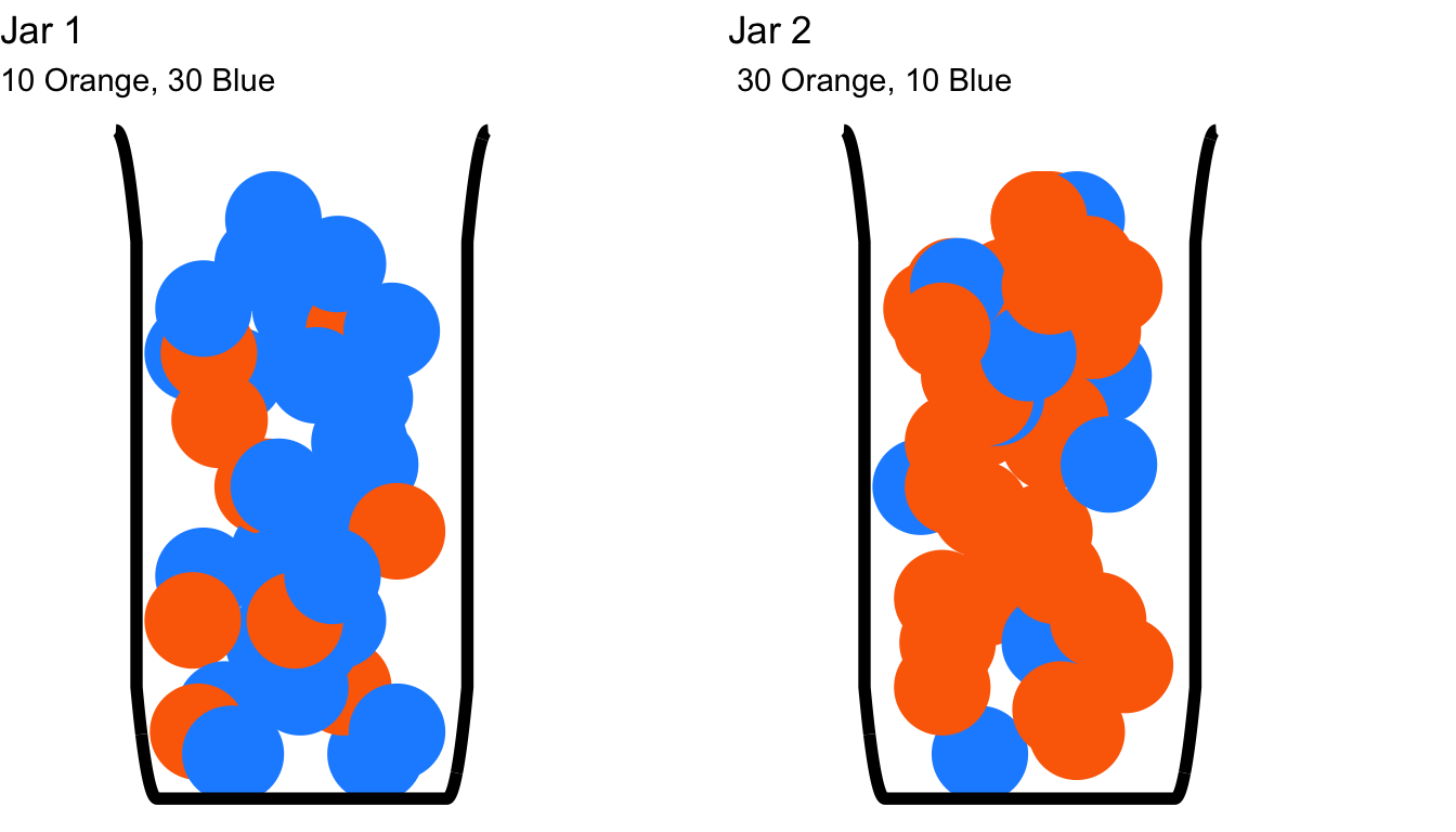
Figure 5.1: Figure 1: A Callback to Some Conditional Probability Problems

The probability that a blue marble was drawn from Jar 1 is 0.75 and the probability that it was drawn from Jar 2 is 0.25: it is three times more probable that the marble came from Jar 1 than from Jar 2.

Now, let’s say we have a jar with a more unusual shape, perhaps something like this…

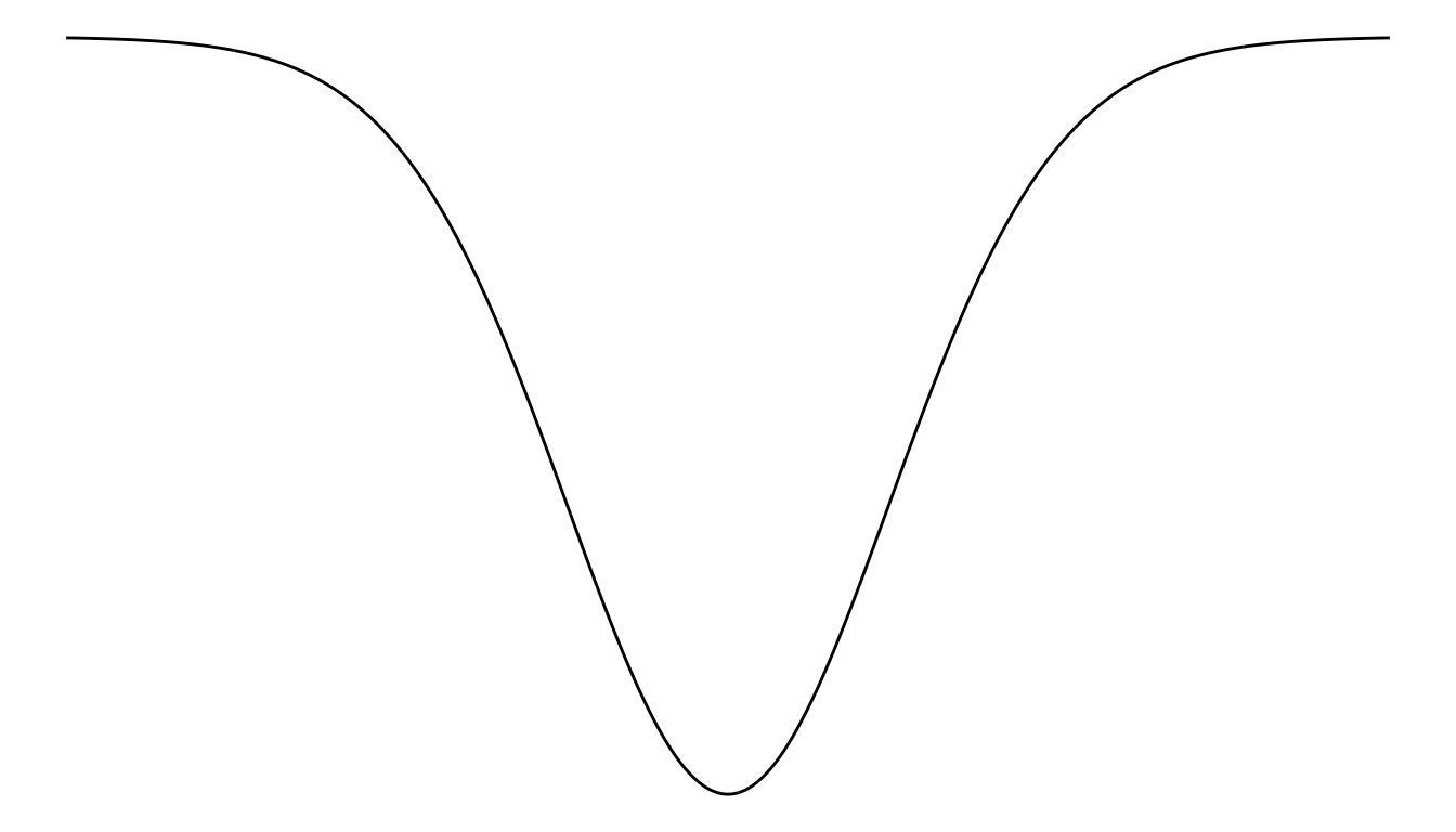
Figure 5.2: Figure 2. An Unusually-shaped Jar

…and the marbles we were interested in weren’t randomly mixed in the jar but happened to sit in the upper corner of the jar in the space shaded in blue…

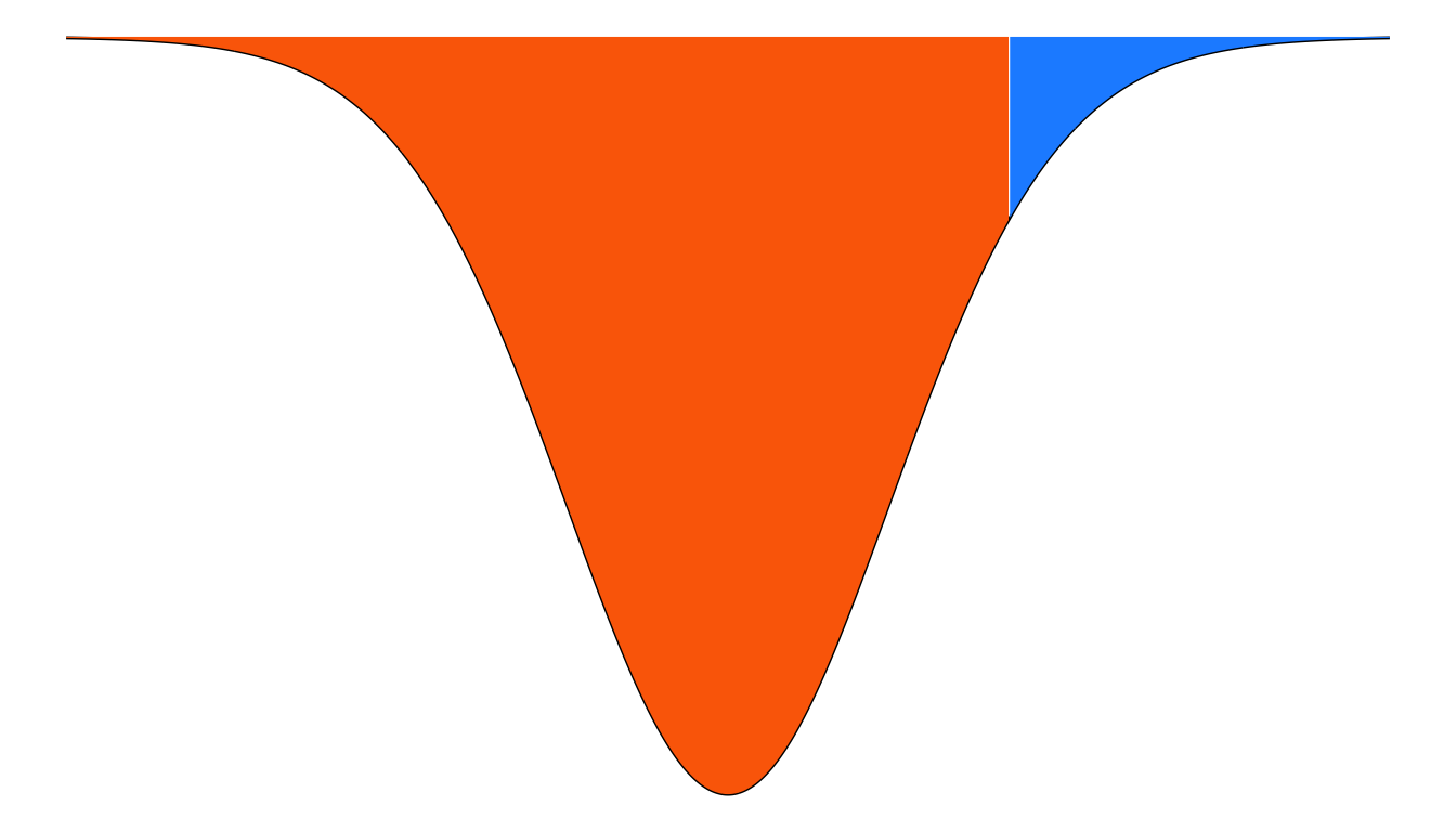
Figure 5.3: Figure 3. Areas of Residence for Interesting Marbles in An Unusually-shaped Jar

…and somehow it were equally easy to reach every point in this jar (the analogy is beginning to weaken). If you were to draw an orange marble from this strange jar, you might think nothing of it. If you were to draw a blue marble, you might think the idea that it came from this jar rather odd. You might even reach a conclusion like the following:

The probability that the blue marble came from that mostly-orange jar is so small that – while there is a small chance that I am wrong about this – I reject the hypothesis that this blue marble came from this jar in favor of the hypothesis that the blue marble came from some other jar.

If we turn that jar upside-down, and we put it on a coordinate plane, then we will have something like this:

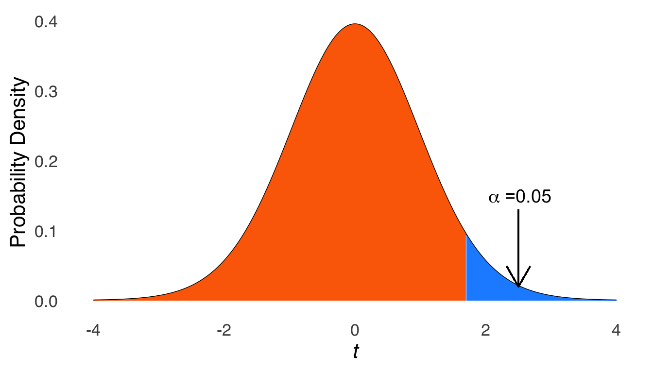
Figure 5.4: Figure 4. Metamorphosis of an Unusually-shaped Jar

Swap out the concept of drawing a marble for observing a sample mean, and this is now a diagram of a one-tailed $t$ test.

The above thought exercise was meant to be the statistical version of this:

This page provides some connection between the marbles and jars (and the coin flips and the dice rolls and the draws of playing cards from well-shuffled decks) and statistical analyses. Frequency distributions are tools that will help us understand the events and sample spaces needed to make probabilistic inferences for statistical analysis.

5.2 The Binomial Distribution

The binomial likelihood formula:

\[p(s|N-s+f, \pi)=\frac{N!}{s!f!}\pi^s(1-\pi)^f\]

was derived in the page on Probability Theory. The binomial likelihood gives the probability of $s$ events of interest (which we have called successes) in $N$ trials where the probability of success on each trial is $\pi$ and $f$ represents the number of trials where success does not occur (i.e., $f=N-s$).

For example, imagine that the manager of a supermarket wants to know what the probability is that shoppers will choose an item placed in the middle of a display (box $B$ in Figure 5.5 below) of three items rather than the items on either side ($A$ or $C$):

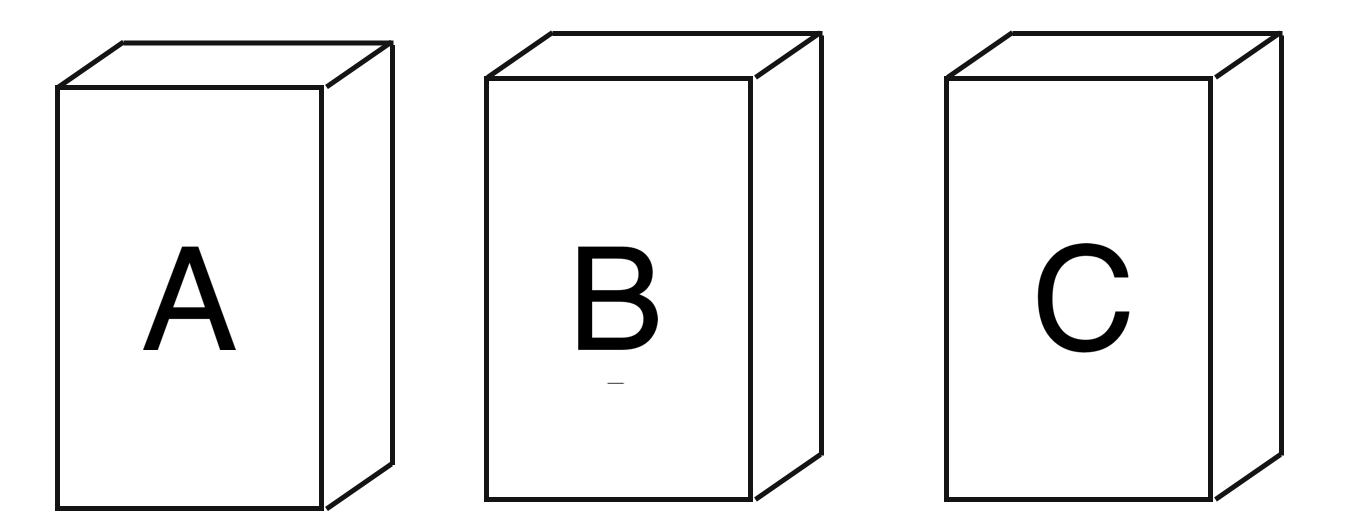
Figure 5.5: Item A, Item B, and Item C

If each item were equally likely to be chosen, then the probability of a person choosing B is $p(B)=1/3$, and the probability of a person choosing not B is $p(\neg B)=p(A\cup C)=1/3+1/3=2/3$. Suppose, then, that 10 people walk by the display. What is the probability that 0 people choose item $B$? That is, what is the probability that $B$ occurs 0 times in 10 trials? According to the binomial likelihood function:

\[p \left(0|\pi=\frac{1}{3}, N=10\right)=\frac{10!}{0!10!} \left( \frac{1}{3} \right)^0 \left( \frac{2}{3} \right)^{10}=0.017\] Were we so inclined – and we are – we could construct a table for each possible number of $s$ given $\pi=1/3$ and $N=10$:

$s$	$p(s\|\pi, N)$
0	0.01734
1	0.08671
2	0.19509
3	0.26012
4	0.22761
5	0.13656
6	0.05690
7	0.01626
8	0.00305
9	0.00034
10	0.00002
$\sum 0 \to 10$	1

These eleven values represent a distribution of values, namely, a binomial distribution. We can represent this distribution as a bar chart with each possible value of $s$ on the $x$-axis and the probability of each $s$ on the $y$-axis:

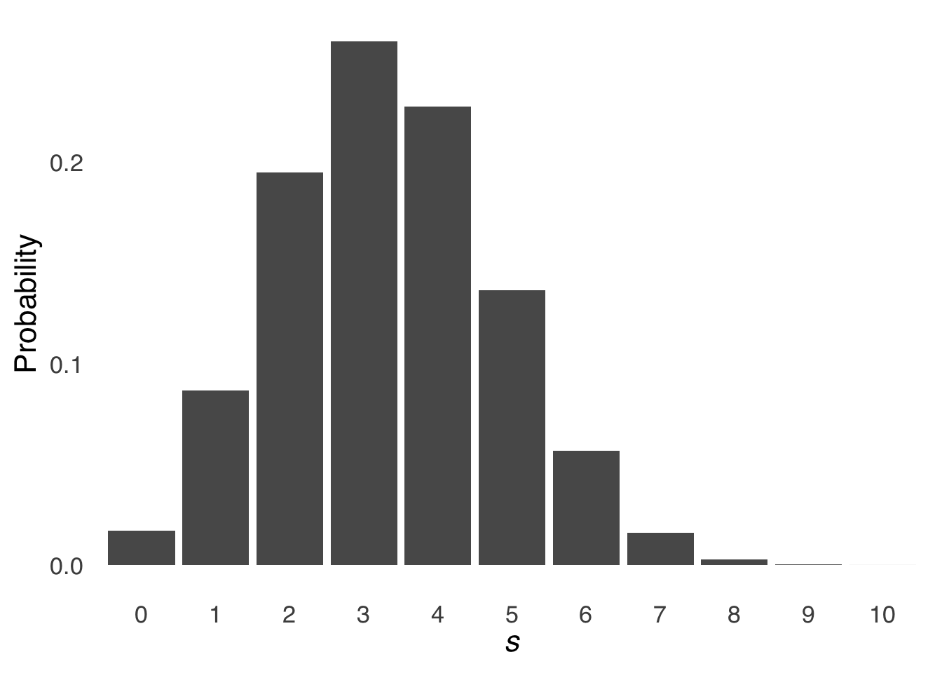
$Binomial Distribution for $N = 10$ and $\pi = 1/3$$

Figure 5.6: Binomial Distribution for $N = 10$ and $\pi = 1/3$

5.2.1 Discrete Probability

The distribution of binomial probabilities listed in Table ?? has eleven distinct values in it, and the visual representation of it in Figure 5.6 comprises eleven distinct bars. The binomial distribution is an example of a discrete probability distribution: each value is an expression of the probability of a discrete event. There are no probability values listed for, say, 2.3 successes or 4.734 successes, because those aren’t feasible events.

5.2.2 Features of the Binomial Distribution

Binomial distributions are positively skewed, like the one in Figure 5.6 above, whenever $\pi$ is between 0 and 0.5, negatively skewed whenever $\pi$ is between 0.5 and 1, and symmetrical whenever $\pi$ is exactly 0.5.¹¹³ The effect of changing $\pi$ is shown below in Figure 5.7. For each distribution represented in Figure 5.7, $N=20$, and the only thing that changes is $pi$.

$The Binomial Distribution for $N = 20$ and Various Values of $\pi$$

Figure 5.7: The Binomial Distribution for $N = 20$ and Various Values of $\pi$

A coin flip is represented by a binomial distribution with $\pi=0.5$ and $N=1$. If we define $s$ as the coin landing heads, then there are two possible values of $s$ – 0 and 1 – and each of those values has a probability of 0.5. If that distribution is represented with an elegant figure such as Figure 5.8, it looks like two large and indistinct blocks of probability. As $N$ grows larger, the blocks become more distinct as more events are possible and have an increasingly large variety of likelihoods.

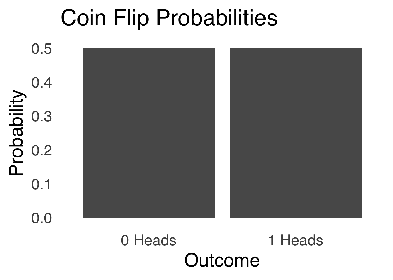
Figure 5.8: Binomial Distribution for a Coin Flip

Figure 5.9 shows a series of binomial distributions each with $\pi=0.5$ and with $N$ ranging between 1 and 20.

$Binomial Distributions for $\pi = 0.5$ and Various Values of $N$$

Figure 5.9: Binomial Distributions for $\pi = 0.5$ and Various Values of $N$

As $N$ gets bigger, the binomial distribution looks decreasingly like the blocky figure representing a coin flip and increasingly like a curve: specifically like a normal curve. That is not a coincidence. In fact, there are meaningful connections between the binomial distribution and the normal distribution, as discussed below

5.2.3 Sufficient Statistics for the Binomial

In Figure 5.7 and Figure 5.9, the binomial changes as a function of $\pi$ and of $N$, respectively. Those are the only two numbers that can affect the binomial distribution and, conversely, they are the only two numbers needed to define a binomial distribution. Thus, they are known as the sufficient statistics¹¹⁴ for the binomial distribution. We can think of the sufficient statistics for a distribution as the numbers we need to know (and the only numbers we need to know) to draw an accurate figure of a distribution. For the binomial distribution, if we know $N$, then we know the range of the $x$-axis of the figure: it will go from $s=0$ to $s=N$. If we know $\pi$ as well, then for each value of $s$ on the $x$-axis, we can calculate the height of each bar on the $y$-axis.

5.2.3.1 Expected Value of the Binomial Distribution

In probability theory, we noted that the expected value of a discrete probability distribution is:

\[E(x)=\sum_{i=1}^N x_i p(x_i)\] and the variance is:

\[V(x)=\sum_{i=1}^N(x_i-\bar{x})^2p(x_i)\]

For the case of the binomial distribution, we showed that:

\[E(x)=\sum_{i=1}^N x_i p(x_i)=N\pi\] It’s a little more complex to derive, but in the end, the variance of a binomial distribution has a similarly simple form:

\[V(x)=\sum_{i=1}^N(x_i-\bar{x})^2p(x_i)=N\pi(1-\pi)\] Thus, the mean of the binomial distribution is $N\pi$, and the variance is $N\pi(1-\pi)$. Please note that those summary statistic formulae apply only for binomial data – it’s just something special about the binomial. Please also note that these equations will come in handy later.

5.2.4 Cumulative Binomial Probability

A cumulative probability is a union probability for a set of events. For example, the probability of rolling a $6$ with a six-sided die is $1/6$; the cumulative probability of rolling $4, 5, or~6$ is $3/6$. Unless otherwise specified, the range of the cumulative probability of $s$ is the union probability of $s$ or any outcome with a value less than $s$. In the case of a discrete probability distribution such as the binomial:

\[Cumulative~p(s)=p(s)+p(s-1)+p(s-2)+...+p(0)\]

That is, for a discrete probability distribution, we get the cumulative probability at event $s$ by adding up all the probabilities $s$ and each possible smaller $s$. We can replace each value in Table ?? – which showed the discrete probabilities for each possible value of $s$ for a binomial distribution with $N=10$ and $\pi=1/3$ – with the cumulative probability for each value of $s$. In Table ??, the cumulative probability for $s=0$ equals the discrete probability for $s=0$ because there are no smaller possible values of $s$ than 0. The cumulative probability for $s=1$ is equal to $p(s=1)+p(s=0)$, the cumulative probability for $s=2$ is equal to $p(s=2)+p(s=1)+p(s=0)$, etc., until the largest possible value of $s$ – $s=10$, where the cumulative probability is 1.*¹¹⁵

$s$	$p(s \le s\|\pi, N)$
0	0.01734
1	0.08671
2	0.19509
3	0.26012
4	0.22761
5	0.13656
6	0.05690
7	0.01626
8	0.00305
9	0.00034
10	0.00002
$\sum 0 \to 10$	1

Figure 5.10 is a chart of the cumulative binomial distribution for $N=20, \pi=1/3$:

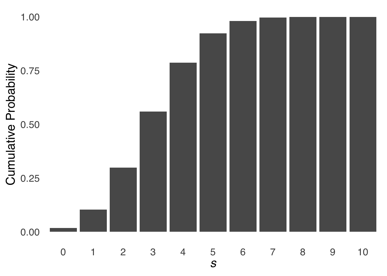
$Cumulative Binomial Distribution for $N = 10$ and $\pi = 1/3$$

Figure 5.10: Cumulative Binomial Distribution for $N = 10$ and $\pi = 1/3$

5.2.5 Finding Binomial Probabilities with R Commands

The binomial likelihood function is relatively easy to type into the R console or to include in R scripts, notebooks, and markdowns. We can translate right-hand side of the binomial equation:

\[p(s|N, \pi)=\frac{N!}{s!f!}\pi^s(1-\pi)^f\] as:

(factorial(N)/(factorial(s)*factorial(f)))*(pi^s)*(1-pi)^f

replacing N, s, f, and pi with the values we need.

But R also has a built-in set of commands to work with several important probability distributions, the binomial included. This set of commands is based around a set of prefixes – indicating the feature of the distribution to be evaluated – a set of roots – indicating the distribution in question – and parameters inside of parentheses. There are a number of helpful guides to the built-in distribution functions in R, and we will have plenty of practice with them.

To find a single binomial probability, we use the dbinom() function. d is the prefix for probability density: we will describe the term “probability density” in more detail in the section on the normal distribution, but for discrete probability distributions like the binomial, the “density” is equal to the probability of any given event $s$. binom is the function root meaning binomial (they’re usually pretty well-named), and in the parentheses we put in $s$, $N$, and $\pi$.

For example, if we want to know $p(s=3|N=10, \pi=1/3)$, we can enter: dbinom(3, 10, (1/3)) which will return 0.2601229.

To find a cumulative probability, we can either add several dbinom() commands or simply use the pbinom() command, where the prefix p indicates a cumulative probability. If we want to know $p(s\le3|N=10, \pi=1/3)$, we can enter: pbinom(3, 10, (1/3)) which will return 0.5592643. By default, pbinom() returns the probability of $s$ or smaller. For the probability of events greater than $s$, we enter the parameter lower.tail=FALSE to our pbinom() parentheses (lower.tail=TRUE is the default, so if we leave it out then lower tail is assumed). Thus, pbinom(3, 10, (1/3)) + pbinom(3, 10, (1/3), lower.tail=FALSE) will return 1. If we want to know the probability of values greater than or equal to 3 using pbinom() and lower.tail=FALSE, then we need to use $s-1$,¹¹⁶ as in: $p(s\ge 3|N=10, \pi=(1/3))$=pbinom(2, 10, (1/3), lower.tail=FALSE).

5.3 The Normal Distribution

We can think of the normal distribution as what happens when the average event is most likely to happen and the likelihoods of other events smoothly decrease as they get farther from that average event. That is: the average is the peak likelihood, and every event to the left or right is just a little bit less likely than the one before.

As a rule, we’re not going to go very deep into Calculus in this course, but if you are interested in the derivation of the functional form of the normal distribution, this article is the easiest-to-follow description that I have encountered.

Here is the form of the function that describes the normal distribution:

\[f(x|\mu, \sigma)=\frac{1}{\sigma\sqrt{2\pi}}e^{-\frac{1}{2}\left(\frac{x-\mu}{\sigma}\right)^2}\]

As equations go, it’s kind of a lot. Please feel free not to memorize it: you won’t need to produce it in this course, and when and if you need to use it in the future, it comes up after a pretty quick internet search. But, while you’re here, I would like to point out a couple of features of it:

The left side of the equation – $f(x|\mu, \sigma)$ – indicates that the normal distribution is a function of $x$ given $\mu$ and $\sigma$.
$x$, $\mu$ and $\sigma$ are the only variables in the equation ($\pi$ is the constant 3.1415… and $e$ is the constant 2.7183…).

Points (1) and (2) together mean that $\mu$ and $\sigma$ (or $\sigma^2$ – it doesn’t really matter because if you know one, then you know the other) are the sufficient statistics for the normal distribution. All you need to know about the shape of a normal distribution are those two statistics. You might ask: what about the skewness and the kurtosis? It’s a good question and the answer is quasitautological¹¹⁷: if the distribution has any skew and/or any excess kurtosis, then it’s not a normal distribution by definition.

The equation describes the probability density at each point on the $x$-axis, not the probability of any point on the $x$-axis.

The probability density is a measure of the relative likelihood of different values: it shows, for example, the peak of the distribution at the mean, and the relatively low likelihoods of the tails. However, at no point on the curve does $f(x)$ (or, $y$) represent a probability in the sense of the probability of an event.

Probability density is a little like physical density¹¹⁸. The density of an object is the mass per unit of area of that object: it’s an important characteristic for certain applications (like, say, building a boat), but if you asked somebody how heavy an object is and they replied with how dense it is, that wouldn’t help you very much. Probability density is the probability per unit of $x$: it’s helpful for a couple of applications but it doesn’t really help us know what the probability of $x$ is. The probability $p(x)$ at any one given point is not equal to $f(x)$ because of the next point.

For any continuous variable $x$, the probability of any single value of $x$ is 0.

This is one of the more counterintuitive facts about probability theory – I think it’s counterintuitive because we seldom think about numeric values as area-less points in a continuous range. Here’s a hopefully-helpful point (ha, ha) to illustrate: please imagine that you are interested in finding the probability that a person selected at random is 30 years old. Based on the proposition described in the previous sentence, we wouldn’t naturally think that the probability is extremely small or even zero: there are lots of people who are 30 years old. Now imagine that you were interested in finding the probability that a person selected at random is 37 years, 239 days, 4 hours, 12 minutes, and 55.43218 seconds old: we would naturally think that that probability would be infinitesimally small, and as the age of interest got even more precise (i.e., more and more digits got added to the right of the decimal on the number of second)

What’s the difference between those two questions? When we’re not in stats class, the phrase 30 years old implies between 30 years and 30 years and 364.9999 days old: the implication is of a range. A range of values can have a meaningful probability. A range of values has an area under the curve, which corresponds to meaningful probability, sort of like how the physical density of an object can be translated into a meaningful mass (or weight) when we know how large the object is. If that’s not clear yet (or even if it is), an illustration of the field of plane geometry might be helpful. In plane geometry, a point has no area. A line has no area, either. But a shape does have an area:

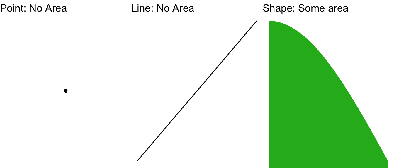
Figure 5.11: A Point, a Line, and a Shape

Having established that there is no probability for a single value of a continuous variable, let’s clarify one potentially-lingering question: why is it that, in the case of the binomial distribution, that there are probabilities associated with single values? The answer is: the binomial distribution is a discrete probability distribution, not a continuous probability distribution. When we find the binomial likelihood of say, $s=4$, we mean $s=4$, not $s=4.0000000$ or $s=4.0000001$. In terms of area, the bars in the visual representation of the binomial distribution have width as well as height: the width of each bar associated with a value of $s$ is 1; so the area is equal to the height of each bar times 1, which simplifies to the height of each bar. We will revisit that fact when we discuss the connections between the normal and the binomial below.

Given that meaningful probabilities for continuous variables are associated with areas, it is reasonable to infer that we should talk about how to find areas under the normal curve, and therefore how to find probabilities. That is true, but there is just one problem:

There is no equation for the area under the normal curve.

Typically, if we want to find the area under a curve, we would use integral calculus to come up with a formula. But, the formula for a normal curve – $f(x|\mu, \sigma)=\frac{1}{\sigma\sqrt{2\pi}}e^{-\frac{1}{2}\left( \frac{x-\mu}{\sigma} \right)^2}$ – is one of those formulas that simply does not have a closed-form integral solution.

But that won’t stop us! Despite not being able to use a formula for the precise integral, we can approximate the area under a curve to a high level of precision. There are two tools available to us to find areas: using software and _calculating areas based using standardized scores.

For example, imagine a standardized test where the average score is 1000 and the standard deviation of the scores is 100: the distribution of scores for this hypothetical test is visualized in Figure 5.12. What is the probability that somebody who took the test that is selected at random scored between 1000 and 1100?

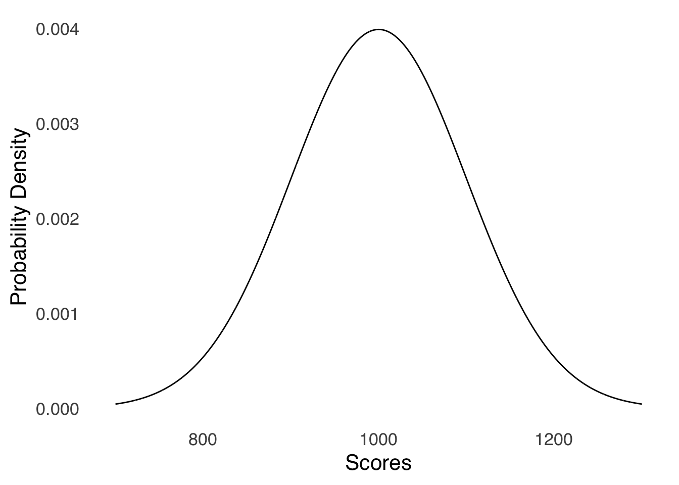
$Distribution of Scores for a Hypothetical Standardized Test With $\mu=1000$ and $\sigma=100$$

Figure 5.12: Distribution of Scores for a Hypothetical Standardized Test With $\mu=1000$ and $\sigma=100$

First, let’s do this with the benefit of modern technology. The absolute easiest way to answer the question is to use an online calculator like this one, where you can enter the mean and standard deviation of the distribution and the value(s) of interest. Slightly, but I don’t think much more, difficult, is to use built-in R functions.

Recall from the discussion of using R’s built-in distribution functions for the binomial that the cumulative probability for a distribution is given by the family of commands with the prefix p. The root for the normal distribution is norm, so we can use the pnorm() function to find probabilities of ranges of $x$ values. The pnorm() function takes the parameter values (x, mean, sd), where x is the value of interest and mean and sd are the mean and standard deviation of the distribution. As with the pbinom() command, the default value for pnorm() is lower.tail=TRUE, so without specifying lower.tail, pnorm() will return the cumulative probability from 0 to $x$¹¹⁹ The mean of this distribution (as given in the description of the problem above) is 1000 and the standard deviation is 100.

Thus, to find the probability of finding an individual with a score between 1,000 and 1,100 where the scores are normally distributed with a mean of 1,000 and a standard deviation of 100, we can use pnorm(1100, 1000, 100) to find the cumulative probability of a score of 1,100 and pnorm(1000, 1000, 100) to find the cumulative probability of a score of 1,000, and subtract the latter from the former:

pnorm(1100, 1000, 100) - pnorm(1000, 1000, 100)

[1] 0.3413447

Figure 5.13 is a visual representation of the math:

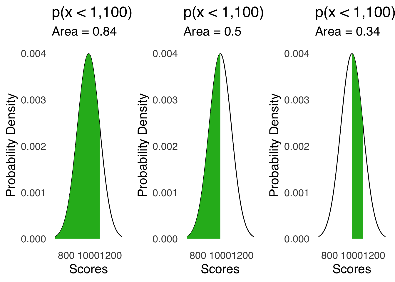
$Visual Representation of Finding the Area Between 1,000 and 1,1000 Under a Normal Curve with $\mu=1000$ and $\sigma=100$$

Figure 5.13: Visual Representation of Finding the Area Between 1,000 and 1,1000 Under a Normal Curve with $\mu=1000$ and $\sigma=100$

The second way to handle this problem – the old-school way – is to solve it using what we know about the area under one specific normal curve: the standard normal distribution. which merits its own section header:

5.3.1 The Standard Normal Distribution

The standard normal distribution is the normal distribution with a mean of 0 and a standard deviation of 1 (the variance is also 1 because $1^2=1$). Here it is right here:

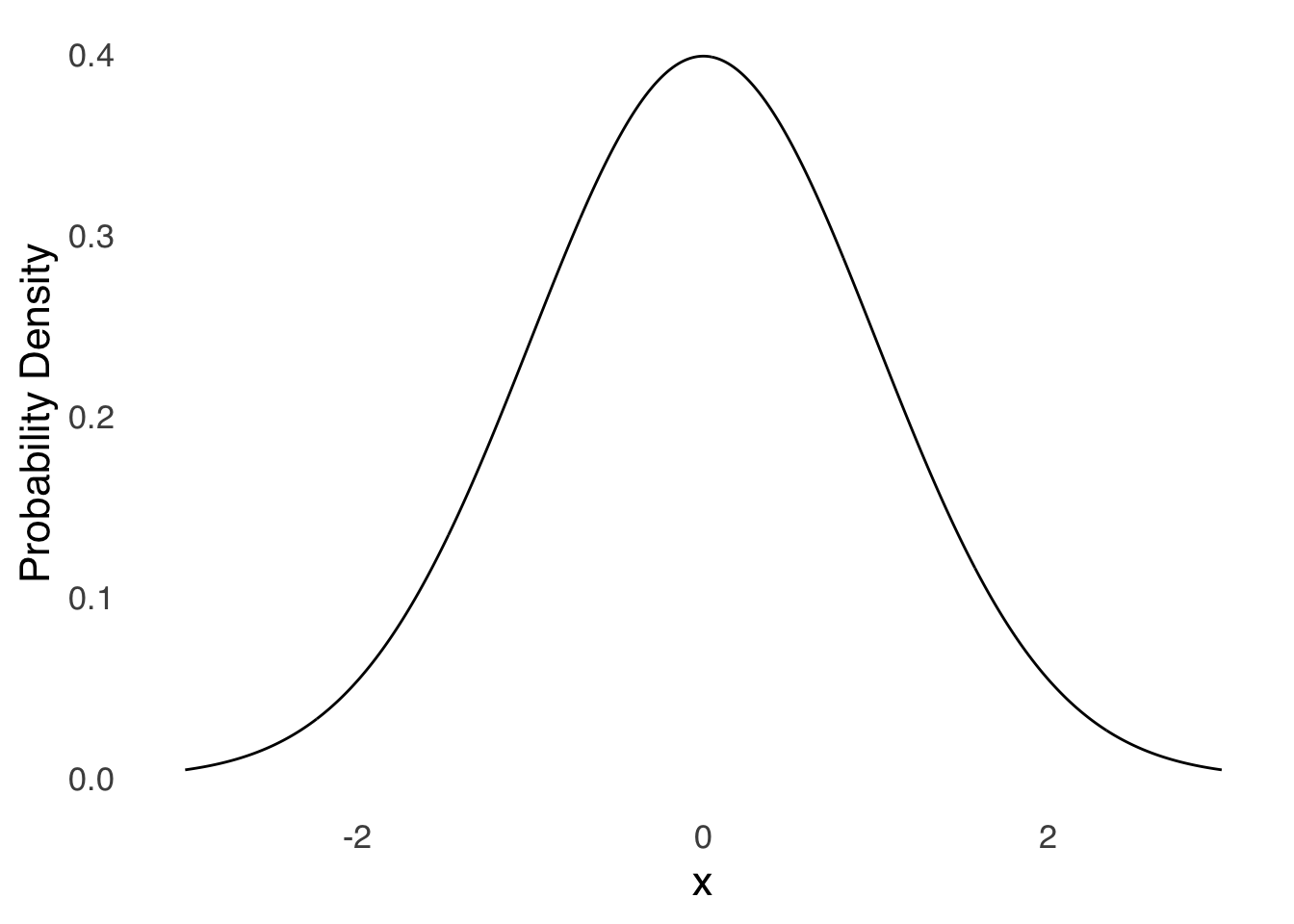
Figure 5.14: The Standard Normal Distribution

The mean and the standard deviation of the standard normal distribution mean that the $x$-axis for the standard normal represents precisely the number of standard deviations from the mean of any value of $x$: $x=1$ is 1 standard deviation above the mean, $x=-2.5$ is 2.5 standard deviations below the mean, etc.. For a long time, the standard normal distribution was the only normal distribution for which areas under the curve were easily available. There are infinite possible normal distributions: one for each possible combination of infinite possible means and infinite possible standard deviations (all greater than 1, but still infinite), and where there is no formula to determine the area under a normal curve, it makes little sense to try take the time to approximate the cumulative probabilities associated for any set of those infinite possibilities. Instead, the cumulative probabilities associated with the standard normal distribution were calculated¹²⁰: if one wanted to know the area under the curve between two points in a non-standard normal distribution, one needed only to know what those two points represented in terms of distance from the mean of that distribution in units of the standard deviation of that distribution. Then, one could (and still can) consult the areas under the standard normal curve to know the area between the $x$ values corresponding to the numbers of standard deviations from the mean. To use our example of standardized test scores – where the mean of the scores is 1,000 and the standard deviation is 100 – a score of 1,100 is one standard deviation greater than the mean, and a score of 1,000 is 0 standard deviations from the mean (it’s exactly the mean). For the standard normal distribution, the area under the curve for $x<1$ – corresponding to a value 1 standard deviation greater than the mean – is 0.84, and the area under the curve for $x=0$ – corresponding to a value at the mean – is 0.5. Thus, since the area under the standard normal curve for $x=0\to x=1$ is $0.84-0.5=0.34$, the area under the normal curve with $\mu=1000 and \sigma=100$ between the mean and a value 1 standard deviation above the mean is also $0.34$.

5.3.1.1 $z$-scores

The value of knowing how many standard deviations from a mean a given value lies in a normal distribution is so important that the distance between any $x$ and the mean in terms of standard deviations is given its own name: the $z$-score. A $z$-score is precisely the number of standard deviations a value is from the mean of a distribution. This is reflected in the $z$-score equation:

\[z=\frac{x-\mu}{\sigma}\]

which is also written:

\[z=\frac{x-\bar{x}}{s}\] when we have the mean and standard deviation of a sample and not the entire population. In other words, we take the difference between any value $x$ of interest and the mean of the distribution and divide that difference by the standard deviation to know how many standard deviations away from the mean that $x$ is.

The $z$-score is important for finding areas under the normal curve using tables like this one, but by “important,” I mean “sort of important but much less important in light of modern technology.” A key note on tables like the one linked: to save space and improve readability, such tables usually don’t include all $z$-scores and full cumulative probabilities, but rather $z$-scores greater than 0 and the cumulative probability between $z$ and the mean and sometimes the cumulative probability between $z$ and the tail (which is to say, to infinity (but not beyond)). To read those tables, one must keep two things in mind: (1) the normal distribution is symmetric and (2) the cumulative probability of either half –below the mean and above the mean – of the standard normal is 0.5 (and thus the total area under the curve is 1).

For example – sticking yet again with the standardized test example – the $z$-score for a test score of 1,100 is:

\[z=\frac{x-\mu}{\sigma}=\frac{1,100-1000}{100}=1\] In the linked table, we can look up $1.00$ in Column A. Column B has the Area to mean for that $z$-score: it’s 0.3413. That means that – for this distribution – 34.13% of the distribution is between the mean and a $z$-score of 1, or, between 1,000 and 1,100. To find the cumulative probability of all values less than or equal to 1,100, we have to add the area that lives under the curve on the other side of the mean, which is 0.5. Thus, the cumulative probability of a score of 1,100 is $0.3413+0.5=0.8413$. The cumulative probability of scores greater than 1,100 is given in Column C: in this case, it’s $0.1587$. Please note that for each row in the table, the sum of the values in Column B and in Column C is 0.5 because the area under the curve on either side of the mean is 0.5. For that reason, some tables don’t include both columns, because if you know one value, you know the other.

Now, what if we were concerned with a score of 900 in a distribution with a mean of 1,000 and a standard deviation of 100? The $z$-score would be:

\[z=\frac{x-\mu}{sd}=\frac{900-1000}{100}=-1\] The negative sign on the $z$-score indicates that the score is less than the mean. The linked table is one of those that doesn’t include negative $z$-scores (as the maker of the table: my deepest apologies). But that’s not a problem because the normal distribution is symmetric: we check Column A for positive 1, and again the area to the mean is 0.3413 and the area to the tail is 0.1587. In this case, the area to the mean is the area under the curve from $-1$ up to the mean, and the area in the tail is the cumulative probability between $-1$ down to negative infinity.

In addition to finding areas under curves – which as noted earlier isn’t quite as important as it used to be given that we can use software to find those areas more easily – the $z$-score is an important tool for making comparisons. Because the $z$-score is a measure for a value of how many standard deviations of its own distribution from the mean of its own distribution, we can use $z$-scores to show how typical or unusual a value is relative to its peer values.

For example, imagine two Girl Scouts – Kimberly from Troop 37 and Susanna from Troop 105 – who are selling cookies to raise funds to facilitate scouting-type activities. Kimberly sells $200 worth of cookies and Susanna sells $175 worth of cookies. We might conclude that Kimberly was the better-performing cookie-seller. However, perhaps Kimberly and Susanna are selling in different markets – maybe Kimberly’s Troop 37 is in a much less-densely populated area and she has fewer potential buyers. In that case, it would make sense to look at the distribution of sales for each troop:

Troop	Mean Sales	SD of Sales
37	$250	$25
105	$150	$10

The $z$-score for Kimberly is $\frac{\$200-\$250}{\$25}=-2$ and the $z$-score for Susanna is $\frac{\$175-\$150}{\$10}=2.5$. Thus, compared to their peers, Susanna outperformed the average by 2.5 standard deviations and Kimberly underperformed the average by 2 standard deviations.

You may have noticed that while the sales numbers for the above examples – the respective sales for Kimberly and Susanna, the means, and the standard deviations – had dollar signs indicating the units of sales, the $z$-scores had no units. In the $z$-score formula, any units that are used cancel out in the numerator and in the denominator. Thus, we can make comparisons between values from distributions with different units, for example: height and weight, manufacturing output and currency value, heart rate and cholesterol level, etc, which really comes in handy when analyzing data with correlation and regression.

5.3.2 Features of the Normal Distribution

As noted above, the normal distribution is always symmetric:

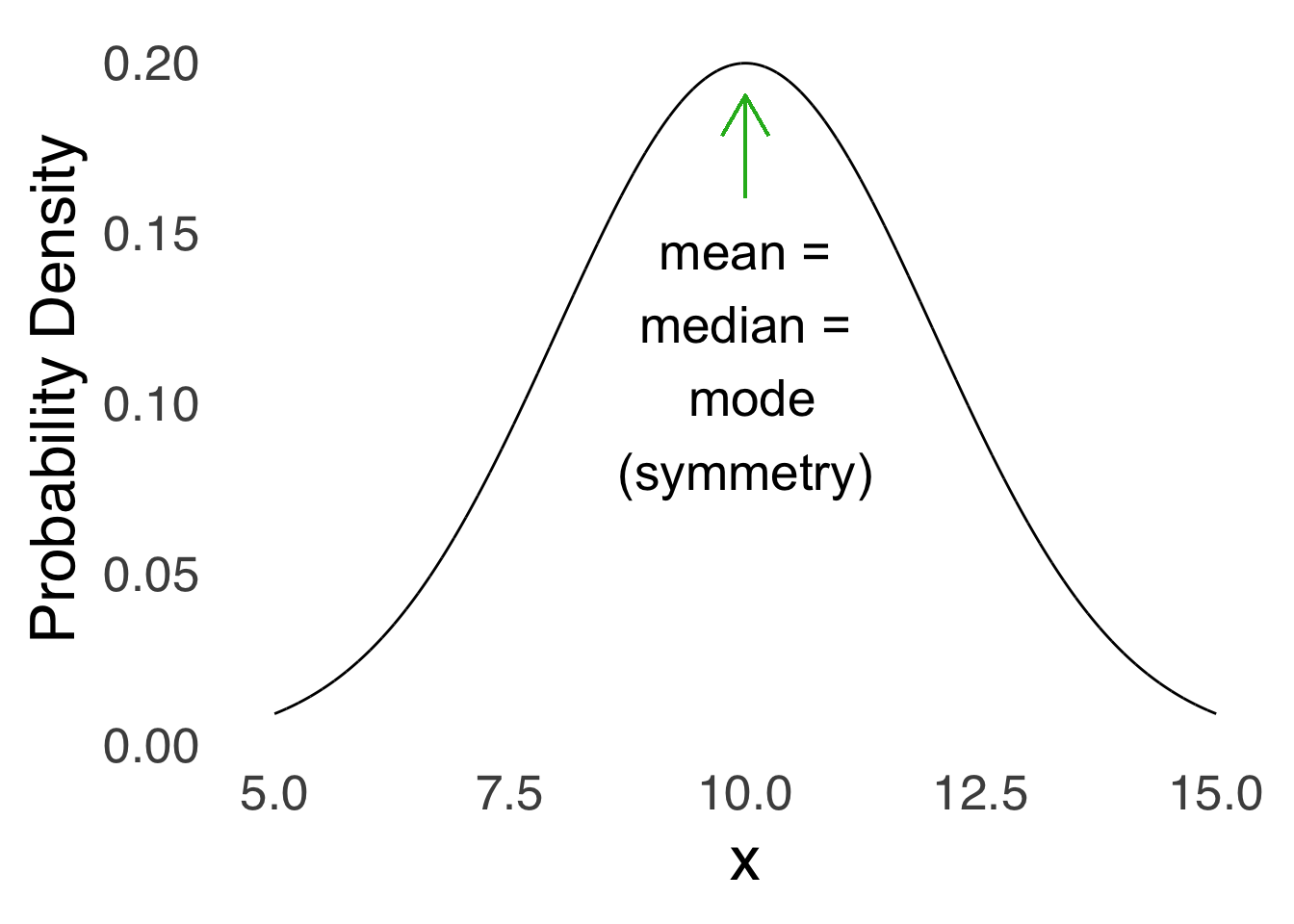
Figure 5.15: Symmetry of the Normal Distribution

The tails of the normal curve come really, really close to touching the $x$-axis but they never touch it. The statistical implication of this is that although the probability of observing values many standard deviations away from the mean can be extremely small, it is never impossible: the normal distribution excludes no values.

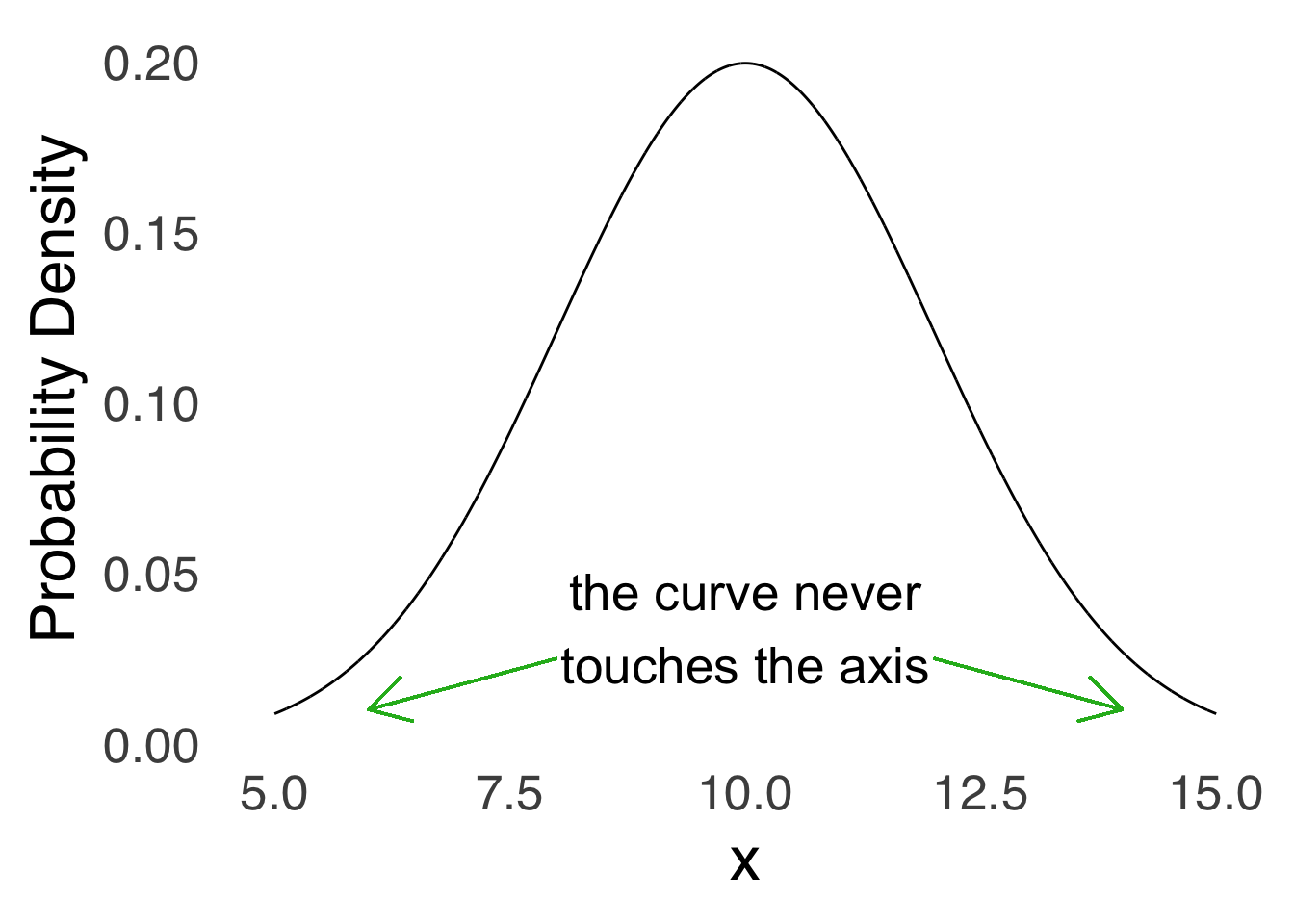
Figure 5.16: The Tails Don’t Touch the Axis

Figure 5.17: Pictured: Kevin Garnett, moments after the conclusion of the 2008 NBA Finals, describing the range of $x$ values in a normal distribution.

The standard deviation – as alluded to in Categorizing and Summarizing Information – is especially important to the normal distribution. It is (along with the mean) one of the two variables in the equation used to draw the curve. It is also the location of the inflection points of the curve: on either side of the mean, the $x$ value that indicates one standard deviation away from the mean is the point where the curve goes from convex down to concave up. The mathematical aspect of that fact isn’t going to play too much in this course, but it is good to know visually where $1 SD$ and $-1 SD$ live on the curve.

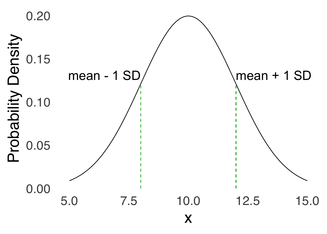
Figure 5.18: Inflection Points of the Normal Curve

The 68-95-99.7 Rule is an old rule-of-thumb that tells us the approximate area under the normal curve within one standard deviation of the mean, within two standard deviations of the mean, and within three standard deviations of the mean, respectively. With all we know about calculating areas under the curves, the 68-95-99.7 rule is less important (we can always look those values up or calculate them with software), but still helpful to know offhand.

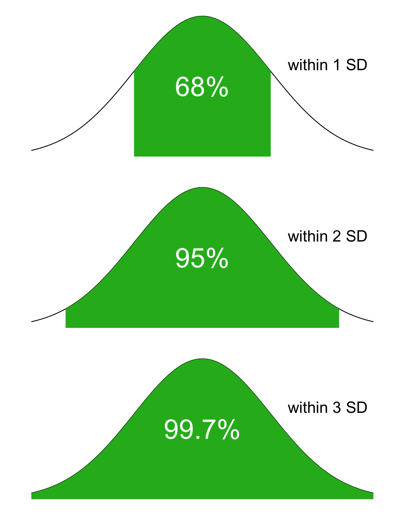
Figure 5.19: The 68-95-99.7 Rule

5.3.3 The Cumulative Normal Distribution

As with the cumulative binomial distribution, the cumulative normal distribution gives at each point the probability of the range of all values up to that point. Also like the cumulative binomial distribution, the cumulative normal distribution starts small and grows to 1 (thanks to the normalization axiom. Unlike the cumulative binomial, the cumulative normal is smooth and continuous. For example, Figure 5.20is a visual representation of the cumulative standard normal distribution. For the case of the cumulative standard normal, please note that the values on the $y$ axis correspond to the areas under the curve for values of $z$.

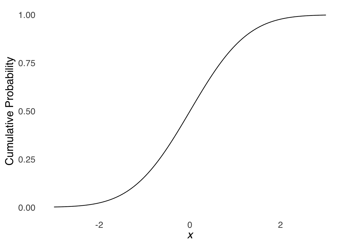
Figure 5.20: The Cumulative Standard Normal Distribution

5.3.4 Percentiles with the Normal Distribution

Percentiles are equal-area divisions of distributions where each division is equal to $1/100$ of the total distribution (for more, see Categorizing and Summarizing Information). For normally-distributed data, the percentile associated with a given value of $x$ is equal to the cumulative probability of $x$, multiplied by 100 to put the number in percent form.

For example, the average height of adult US residents assigned male at birth is 70 inches, with a standard deviation of 3 inches, and the distribution of heights is normal. If we wanted to know the percentile of height among adult US residents assigned male at birth for somebody who is 6’2 – or 74 inches – tall, we would take the cumulative probability of 74 in a normal distribution with a mean of 70 and a standard deviation of 3 either by using software:

pnorm(74, 70, 3)

[1] 0.9087888

Or by finding the $z$-score and using a table:

\[z_{74}=\frac{74-70}{3}=1.33\]

\[Area~to~mean(1.33)=0.4082\] \[Total~area=Area~to~mean+Area~beyond~mean=0.4082+0.5=0.9082\] Then, we multiply the area by 100 and round to the nearest whole number (these things are typically rounded) to get 91: an adult US resident assigned male at birth who is 6’2” is in the 91st percentile for height. They are taller than 91% of people in their demographic category.

5.3.5 The Connections Between the Normal and the Binomial

As noted earlier, the normal distribution and the binomial distribution are closely related. In fact, the limit of the binomial distribution as $N$ goes to infinity is the normal distribution. But, before we get to infinity, the normal distribution approximates the binomial distribution. The rule-of-thumb is that the normal approximation to the binomial can be used when $N\pi>5$ and $N(1-\pi)>5$: that is, the binomial distribution looks enough like the normal given some combination of large $N$ and $\pi$ in the middle of the range (small $N$ makes the binomial blocky; $pi$ near 0 or 1 makes the binomial more skewed).

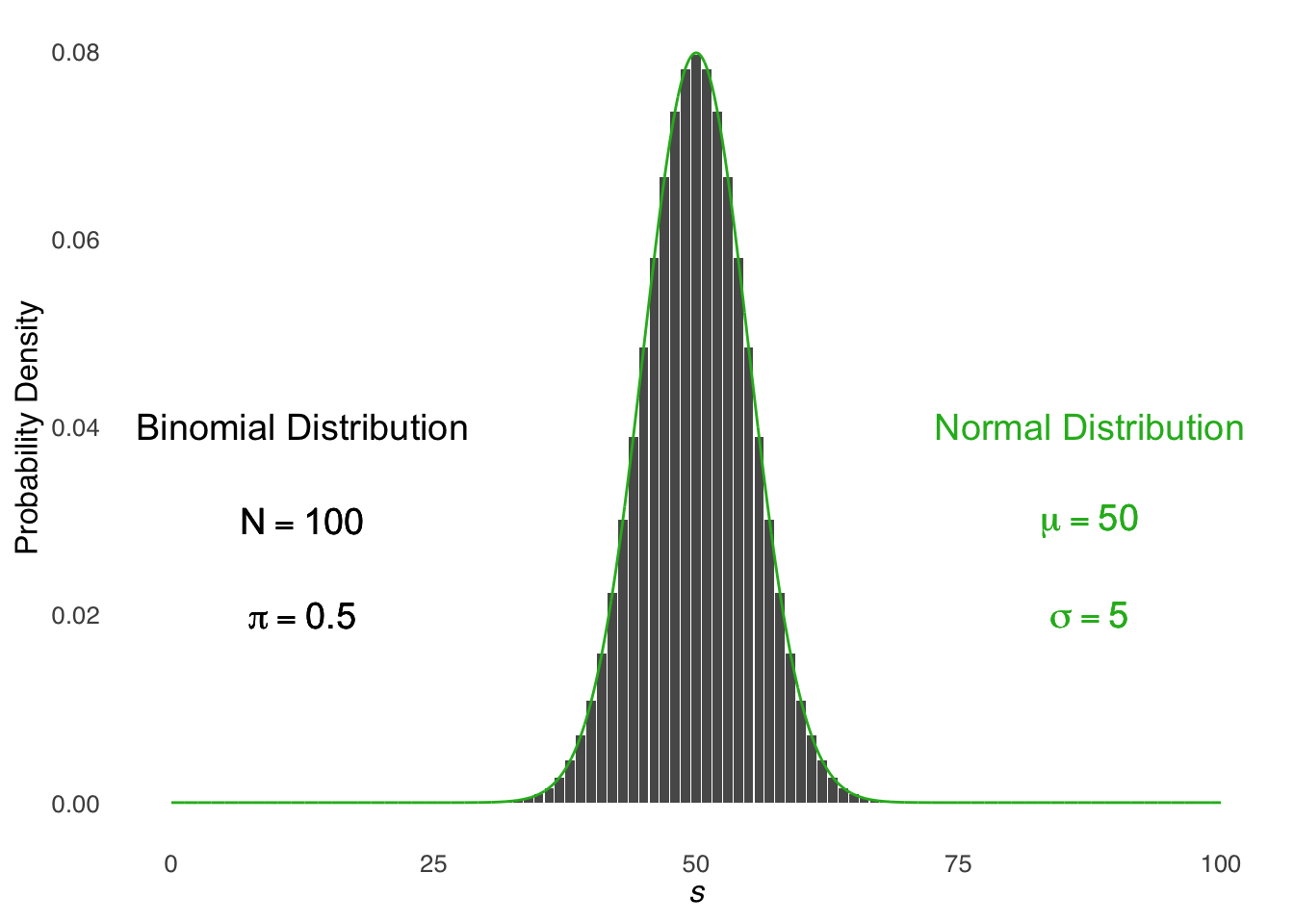
Figure 5.21: Illustration of the Normal Approximation to the Binomial

We know that the mean of a binomial distribution is given by $N\pi$, that the variance is given by $N\pi(1-\pi)$, and that the standard deviation is given by $\sqrt{N\pi(1-\pi)}$. When we use the normal approximation to the binomial, we treat the binomial distribution as a normal distribution with those values for the mean and standard deviation.

For example, suppose we wanted to know the probability of flipping 50 heads in 100 flips of a fair coin (as represented in Figure 20 above). We could simply use software to compute the binomial probability¹²¹, or, we could treat $s=100$ as a value under the curve of a normal distribution with a mean of $N\pi=50$ and a standard deviation of $\sqrt{N\pi(1-\pi)}=5$. Except: there is no probability for a single value in a continuous distribution like the normal as there is for a discrete distribution like the binomial. Instead, we must apply a range to the value of interest: we will give the range a width of $1$ to represent that we are looking for the probability of 1 discrete value and we will use $s$ – in this case $s=50$ – as the midpoint of that range. Thus, to find the approximate binomial probability for $s=50|N=100, \pi=0.5$, we will find the area under the normal curve between $x=49.5$ and $x=50.5$:

\[p(s=50|N=100, \pi=0.5)\approx Area(z_{50.5})-Area(z_{49.5})\] \[=Area \left( \frac{50.5-50}{5}\right)-Area \left( \frac{49.5-50}{5} \right)=0.0797.\] The exact probability for 50 heads in 100 flips is dbinom(50, 100, 0.5) = 0.796, so this was a pretty good approximation.

5.4 the $t$ distribution

The $t$ distribution describes fewer variables than the normal or the binomial, but what it does describe is essential to statistics in the fields of behavioral science. The $t$ distribution is a model for the distribution of sample means in terms of standard errors of the mean.

A sample mean is, as noted in Categorizing and Summarizing Information, the mean of a sample of scores. Any time a psychologist runs an experiment and takes a mean value of the dependent variable for a group of participants, that is a sample mean. Any time an ecologist takes soil samples and measures the average concentration of a mineral in the samples, that is a sample mean.

Sample means have a remarkable property: if you take enough sample means, then the distribution of those sample means will have a mean equal to the mean of the population that the data were sampled from and a variance equal to the variance of the original population divided by the size of the samples. That property is codified in the central limit theorem.

5.4.1 The Central Limit Theorem

The central limit theorem is symbolically represented by the equation:

\[\bar{x} \sim N \left(\mu, \frac{\sigma^2}{n}\right)\]

$\bar{x}$ represents sample means. The tilde (~) in this case stands for the phrase is distributed as. The $N$ means a normal with its mean and variance indicated in the parentheses to follow. $\mu$ is the mean of the population the samples came from, $\sigma^2$ is the variance of the population the samples came from, and $n$ is the number of observations per sample. Put together, the central limit theorem says:

As the size of sample means becomes large, sample means are distributed as a normal with the mean equal to the population mean and the variance equal to the population variance divided by the number in each sample.

And here’s a really wild thing about the central limit theorem:

Regardless of the shape of the parent, the sample means will arrange themselves symmetrically. For positively-skewed distributions, there will be lots of samples from the heavy part of the curve but the values of those sample will be small; there will be few samples from the light part of the curve but the values of those samples will be large. It all evens out eventually.

In a scientific investigation that collects samples, it’s important to know which samples are ordinary and which are extreme (this will be covered in greater detail in Differences Between Two Things). Just as there are infinite possible normal distributions, there are infinite possible distributions of sample means. Likewise, as we got the Standard Normal Distribution by dividing differences of values from the mean by the standard deviation, we get the $t$ distribution by dividing the difference between sample means and the mean of the parent distribution by the standard error (the square root of the sample mean variance $\sigma^2/n$:

\[t=\frac{\bar{x}-\mu}{\sqrt{\frac{\sigma^2}{n}}}=\frac{\bar{x}-\mu}{\frac{\sigma}{\sqrt{n}}}\]

The shape of the $t$ distribution – the model for the distribution of the $t$ statistic – is given by the following formula:

\[f(t)=\frac{\Gamma \left(\frac{\nu+1}{2} \right)}{\sqrt{\nu\pi}~\Gamma \left(\frac{\nu}{2} \right)} \left( 1+\frac{t^2}{\nu} \right)^{-\frac{\nu+1}{2}}\] which, super-yikes, but it does show us that there is only one variable other than $t$ in the equation: $\nu$, also known as degrees of freedom ($df$). That means that the $df$ is the only sufficient statistic for the $t$ distribution.¹²² The mean of the $t$ distribution is 0, and the variance of the $t$ is undefined for $df\le 1$, infinite for $1<df \le 2$, and $\frac{df}{df+2}~for~df>2$.

The $df$ for a sample mean with sample size $n$ is $n-1$. An important caveat (which, admittedly, I glossed over in the text above) is the distribution of sample means approaches a normal distribution as the size of the samples $n$ gets large. “Large” is a relative term: there is no magical point¹²³, but when $df$ gets around 100, the $t$ distribution is almost exactly the same as a normal distribution. For smaller samples, the distribution of $t$ is much more kurtotic, reflecting the fact that it is more likely to get extremely small or large sample means for samples comprising fewer observations. Figure 5.22 shows how the $t$ distribution changes as a function of $df$.

Figure 5.22: The $t$ Distribution for Selected Values of $df$

5.5 The $\chi^2$ Distribution

The $\chi^2$ distribution is used to model squared differences from means. Figure 5.23 provides an illustration: the distribution of deviations from the mean of a standard normal distribution – which is just a standard normal distribution because the mean of the standard normal is 0 – is shown in the upper-left plot. The upper-right plot is the distribution of a set of the deviations from the mean of a standard normal squared (that is, taking each number in a standard normal, subtracting the mean, and squaring the result). The bottom-left plot is the distribution of the sum of two squared deviations from a normal (taking two numbers from a standard normal, subtracting the mean from each, squaring the result for each, and adding them together), and the lower-right plot is the distribution of the sum of three squared deviations from the mean.

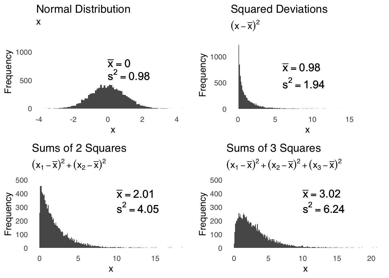
Figure 5.23: A Standard Normal Distribution and its Squared Deviations

The three plots based on squared deviations can be modeled by $\chi^2$ distributions with 1, 2, and 3 $df$, respectively. The degrees of freedom we cite when talking about shapes of the $\chi^2$ distribution are based on the same idea as the degrees of freedom we cite when talking about shapes of the $t$ distribution: both are representations of things that are free to vary. When we are talking about sample means, the things that are free to vary are the observed values in a sample: if we know the sample mean, and we know all values of the sample but one and the sample mean, then we know the last value and thus $n-1$ values in the sample are free to vary but the last one is fixed. When we are talking about the $\chi^2$ distribution, we are talking about degrees of freedom with regard to group membership: if, for example, we have two groups and people have freely sorted themselves into one group, then we know what group the remainder of the people must be in (the other one), so the degrees of freedom for groups in that example is 1. Much more on that concept to come in Differences Between Two Things.

The equation for the probability density of the $\chi^2$ distribution is:

\[f(x; \nu)=\left\{ \begin{array}{ll} \frac{x^{\frac{\nu}{2}-1}e^{-\frac{x}{2}}}{2^{\frac{k}{2}}\Gamma \left(\frac{k}{2} \right)} & \mbox{if } x > 0 \\ 0 & \mbox{if } x \le 0 \end{array} \right.\]

Like the $t$ distribution, the only sufficient statistic for the $\chi^2$ distribution is $\nu=df$. The mean of the $\chi^2$ distribution is equal to its $df$, and the variance of the $\chi^2$ distribution is $2df$.

$\chi^2$ Distributions for Various $df$

Figure 5.24: $\chi^2$ Distributions for Various $df$

Because the $\chi^2$ distribution is itself based on squared deviations, it is the ideal distribution for statistical analyses of squared deviation values. Two of the most important statistics that the $\chi^2$ distribution models are:

Variances. Recall from Categorizing and Summarizing Information that the equation for a population variance is $\frac{\sum(x-\mu)^2}{N}$ and the equation for a sample variance is $\frac{\sum(x-\bar{x})^2}{n-1}$. In both equations, the numerator is a sum of squared differences from a mean value. Thus, the variance is a statistic that is modeled by a $\chi^2$ distribution.
The $chi^2$ statistic. Seems kind of obvious that the $chi^2$ statistic is modeled by the $\chi^2$ distribution, doesn’t it? In the $\chi^2$ tests – the $\chi^2$ test of statistical independence and the $chi^2$ goodness-of-fit test, both of which we will be discussing at length later – the test statistic is:

\[\chi^2_{obs}=\frac{\sum(f_o-f_e)^2}{f_e}\] where $f_o$ is an observed frequency and $f_e$ is an expected frequency. Again, we’ll go over the details of those tests later, but look at that numerator! It’s a squared difference from an expected value, and that is the $\chi^2$’s time to shine, baby!

5.6 Other Probability Distributions

5.6.1 Uniform distribution

A uniform distribution is any distribution where the probability of all things is equal. A uniform distribution can be discrete, as in the distribution of outcomes of a roll of a six-sided die:

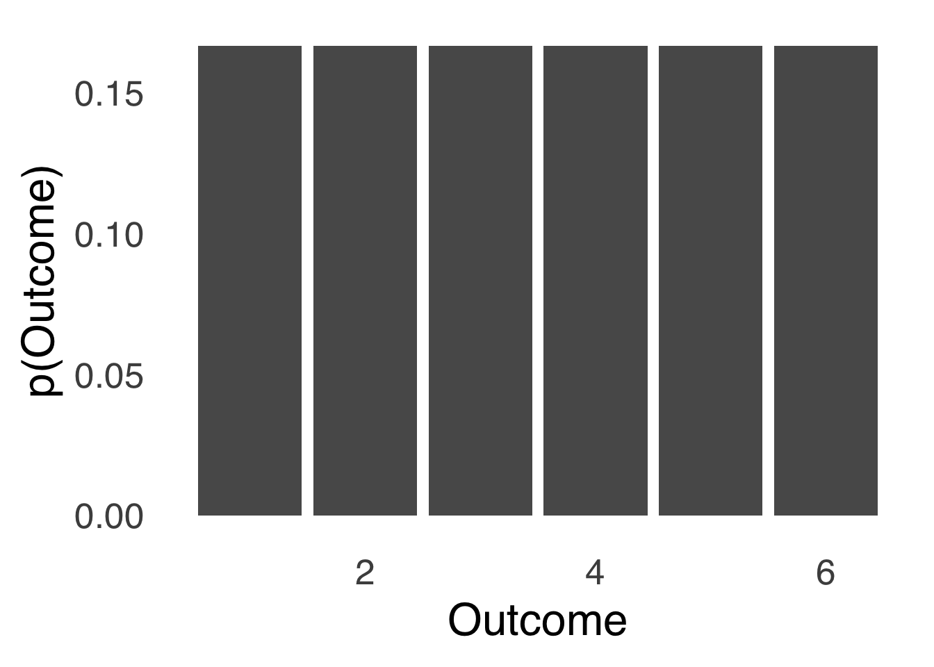
Figure 5.25: A Discrete Uniform Distribution

or it can be continuous, as in the distribution of times in an hour:

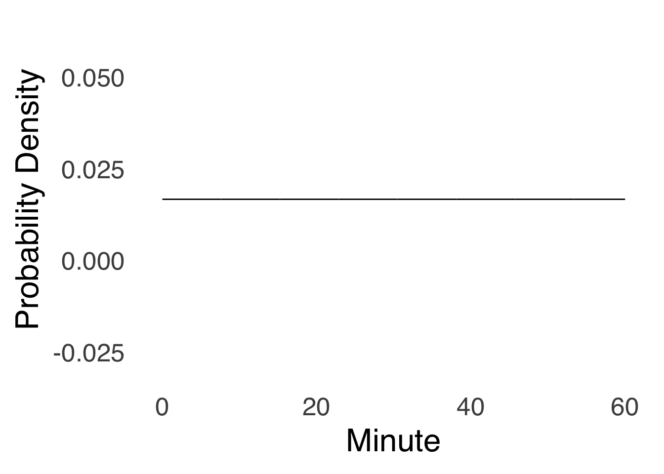
Figure 5.26: A Continuous Uniform Distribution

5.6.2 the $\beta$ distribution

The $beta$ distribution describes variables in the [0, 1] range. It is particularly ideal for modeling proportions. In the terms of the binomial distribution that we have been using, the mean value for a proportion – symbolized $\hat{\pi}$ – is equal to $s/N$. We can also assess the distribution of a proportion based on observed data¹²⁴ in terms of the $\beta$ distribution.

For proportions, the $\beta$ distribution is directly related to the observed successes ($s$) and failures ($f$):

\[mean(\beta)=\frac{s+1}{s+f+2}\]

\[variance(\beta)=\frac{\hat{\pi}(1-\hat{\pi})}{s+f+3}=\frac{(s+1)(f+1)}{(s+f+2)^2(s+f+3)}\]

Figure 5.27 is a visualization of a $\beta$ distribution where $s=4$ and $f=5$. The $\beta$ can be skewed positively (when $s<f$), can be skewed negatively (when $s>f$), or be symmetric (when $s\approx f$).

$A $\beta$ Distribution with $s=4, f=5$$

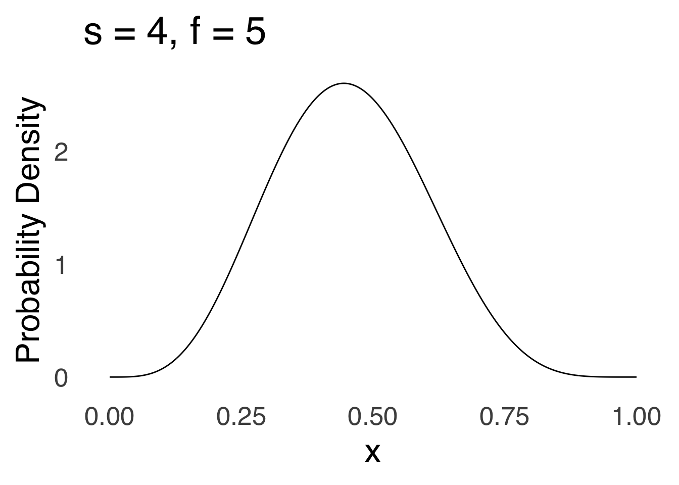
Figure 5.27: A $\beta$ Distribution with $s=4, f=5$

5.6.2.1 The Dirichlet Distribution

The Dirichlet Distribution is to multinomial data what the $\beta$ distribution is to binomial data: in terms of visualization, we can think of it as a “3D $\beta$”. It may or may not come up again but it is a good excuse to include this cool plot:

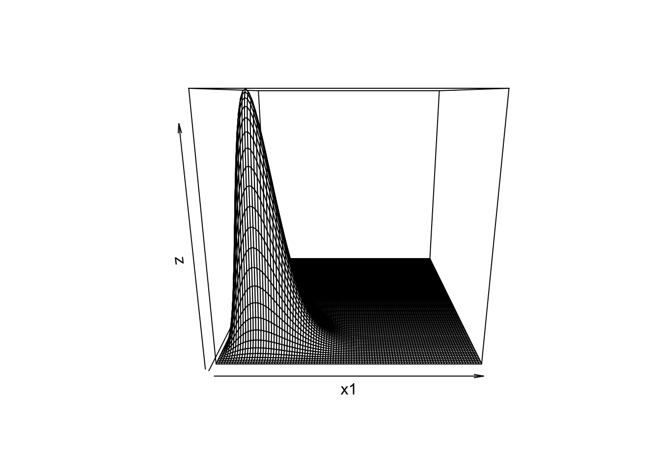
Figure 5.28: Dirichlet Distribution with Shape Parameters 3, 5, 12

5.6.3 The Logistic Distribution

The Logistic Distribution is a model used for probabilities of events. For example, Figure 5.29 represents the number of points scored in NBA games on the $x$ axis and the proportion of times that the team scoring that number of points won the game (the data are restricted only to home teams: otherwise pairs in the data would be closely related to each other):

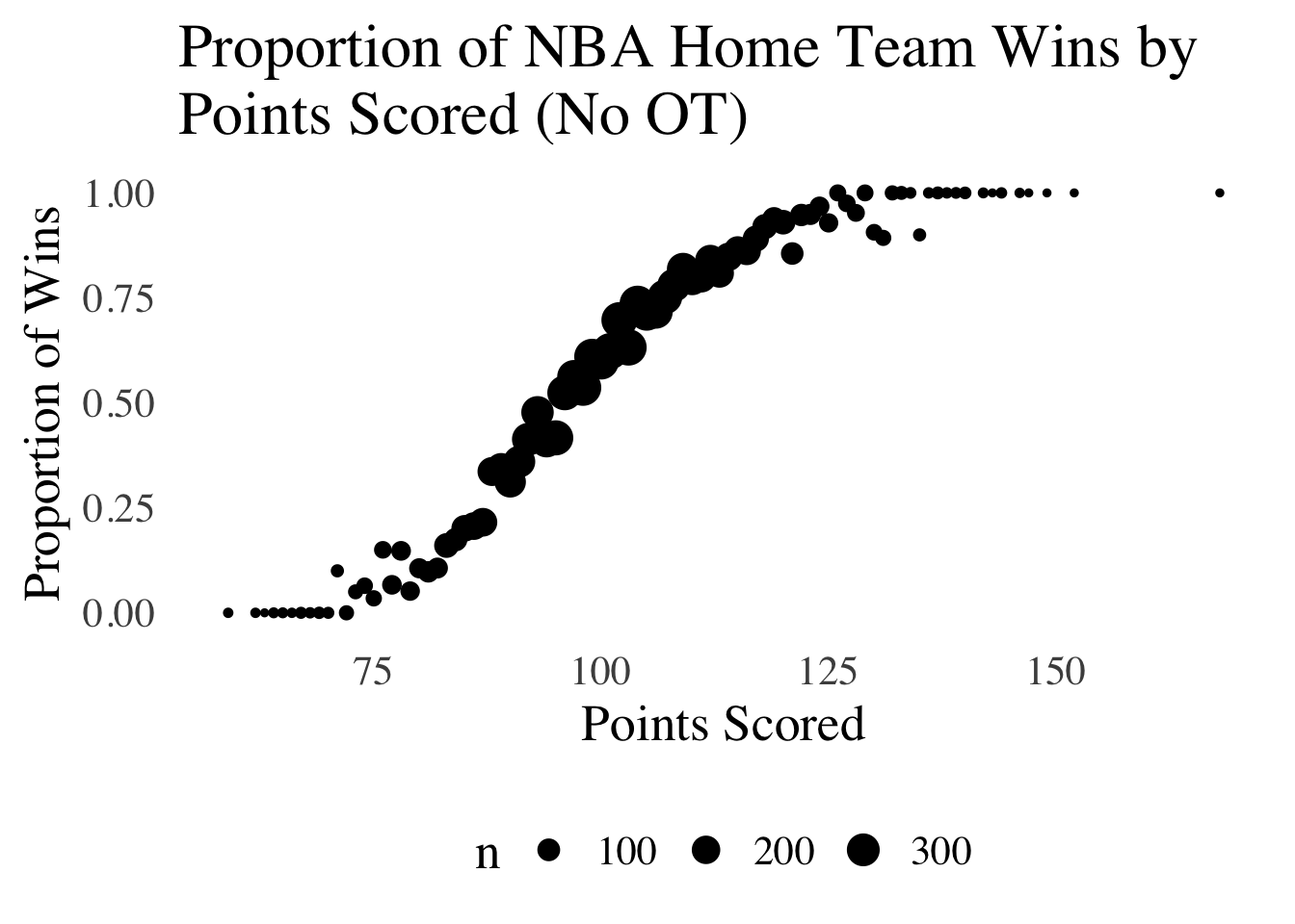
Figure 5.29: Relative Probabilities of Binary Events, Modelable by a Logistic Distribution.

The relative frequency of wins is low for teams that score fewer than 75 points, rises for teams that score between 75 and 125 points, and at 150 points, victory is almost certain. This type of curve is well-modeled by the logistic distribution:

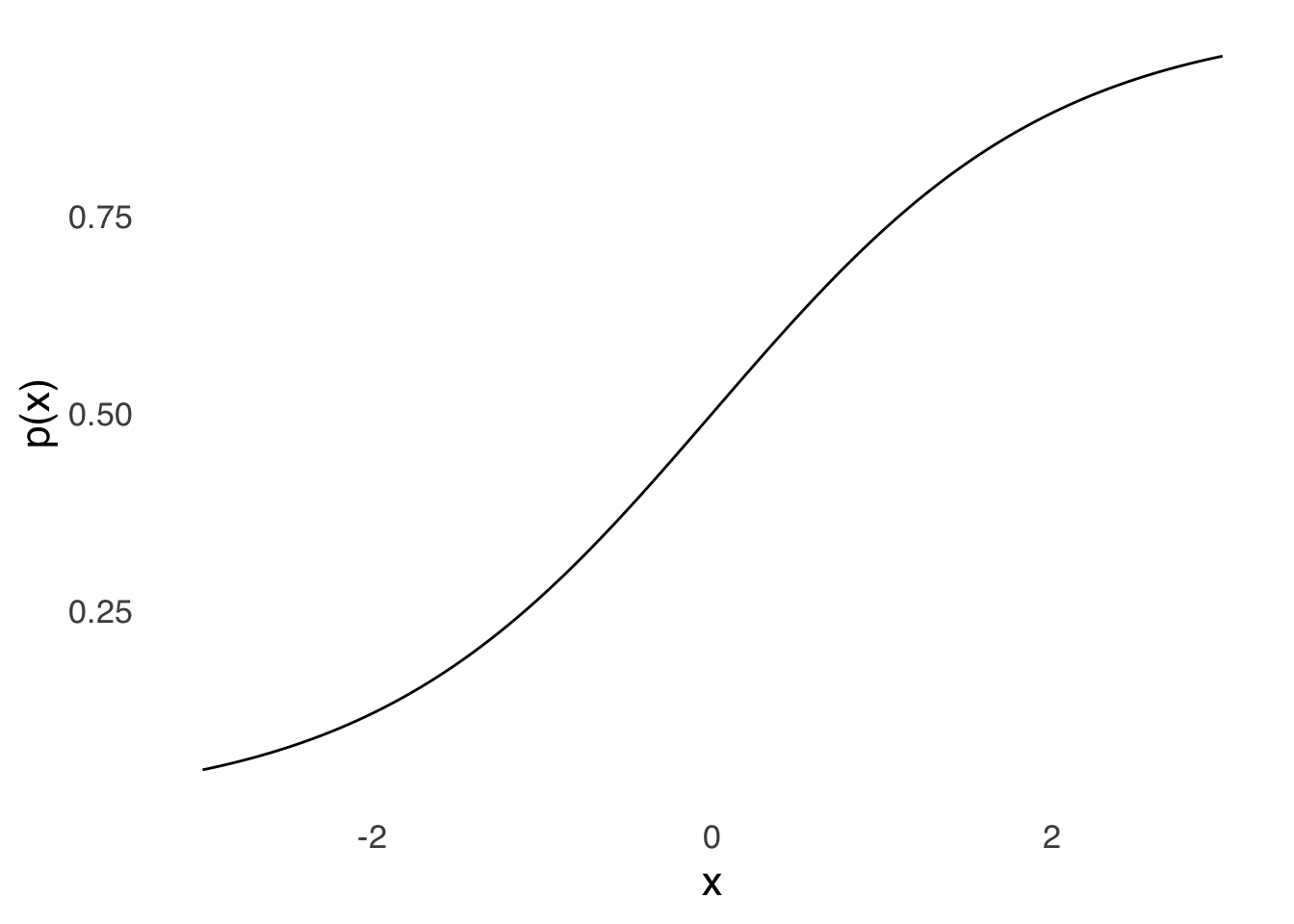
Figure 5.30: The Logistic Distribution

The logistic distribution closely resembles the cumulative normal distribution. Both distributions can be used to model the probability of binary outcomes (like winning or losing a basketball game) based on predictors (like number of points scored) and both are used for that purpose. However, the logistic distribution has some attractive features when used in regression modeling that lead many – myself included – to prefer it.

5.6.4 The Poisson Distribution

The Poisson Distribution models events with predominantly small counts. The classic example of the Poisson Distribution being used to model events is Ladislaus Bortkiewicz’s 1898 book The Law of Small Numbers, in which he described the (small) numbers of members of the Prussian Army who had been killed as a result of horse and/or mule kicks.

It may resemble the Binomial Distribution, and that is no coincidence: the Poisson is a special case of the class of distributions known as the Negative Binomial, which is the distribution of the probability of a number of $s$ occurring before a specified number of $f$ occur.

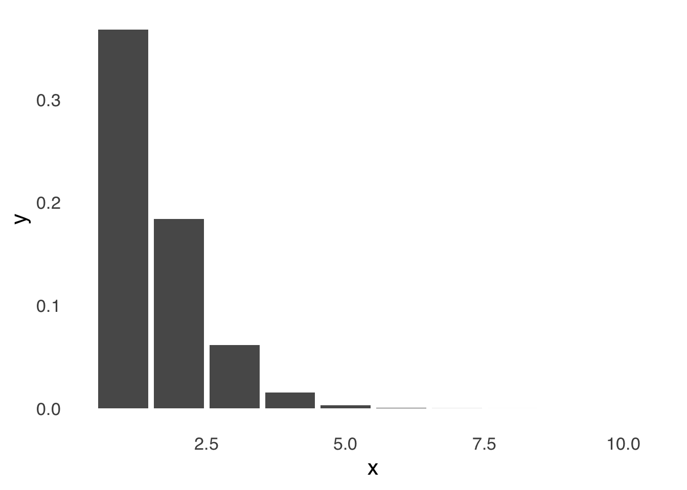
Figure 5.31: The Poisson Distribution

5.7 Interval Estimates

Interval estimates are important tools in both frequentist statistics (as in confidence intervals) and Bayesian statistics (as in credible intervals or highest density intervals). For continuous distributions, interval estimates are areas under the curve.

Figure 5.32 is a visualization of interval estimates for the central 95% under a standard normal distribution, a beta distribution with $s=5$ and $f=2$, a $\chi^2$ distribution with $df=3$, and a $t$ distribution with $df=10$.

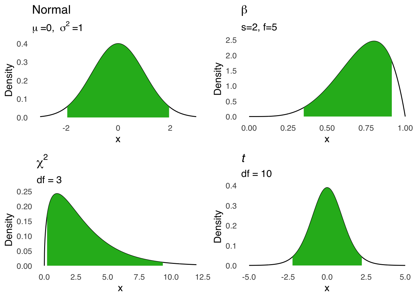
Figure 5.32: Visual Representations of 95% Intervals for Selected Probability Distributions

To find the central 95% interval under each curve, we can use the distribution commands in R with the prefix q for quantile. In each q command, we enter the quantile of interest plus the sufficient statistics for each distribution (we can leave out the mean and sd for the normal command because the default is the standard normal).

Distribution	Lower Limit Command	Lower Limit Value	Upper Limit Command	Upper Limit Value
Normal	qnorm(0.025)	-1.9600	qnorm(0.975)	1.9600
$\beta (s=4, f=1)$	qbeta(0.025, 5, 2)	0.3588	qbeta(0.975, 5, 2)	0.9567
$\chi^2 (df=3)$	qchisq(0.025, 3)	0.2158	qchisq(0.975, 3)	9.3484
$t (df=10$	qt(0.025, 10)	-2.2281	qt(0.975, 10)	2.2281

*Unless your research happens to be about marbles, the jars in which they reside, and the effect of removing them from their habitat, in which case: you’ve learned all you need to know, and you’re welcome.↩︎
If $\pi$ is exactly 0 or exactly 1, there really is no distribution: you would either have no $s$ or all $s$.↩︎
Sufficient Statistics: the complete set of statistical values needed to define a probability distribution↩︎
*The maximum cumulative probability for any distribution is 1.↩︎
The fact that you have to use $s-1$ for cumulative probabilities of all values greater than $s$ is super-confusing and takes a lot of getting used to.↩︎
Strong chance I just made up the word “quasitautological” but let’s go with it.↩︎
Between this and the method of moments, it should be apparent that early statisticans were super into physics and physics-based analogies.↩︎
Unlike the pbinom() command, we don’t have to change $x$ when we go from lower.tail=TRUE to lower.tail=FALSE because $p(x)=0$ for the continuous distributions and so the distinction between $>x$ and $\ge x$ is meaningless.↩︎
As with any mention of R.A. Fisher, it feels like a good to remind ourselves that Fisher was a total dick.↩︎
Well, now we can compute it. The normal approximation was a bigger deal when computers weren’t as good and using formulas with numbers like $100!$ was impossible to do with calculators.↩︎
There are variations on the $t$ that have other parameters. Let’s not worry about them for now.↩︎
Fisher, who again, was a total dick, proposed that samples of at least 30 could be considered to have their means distributed normally, and statistics texts since then have reported 30 as the magic number. It’s just an approximate rule-of-thumb designed for a world without calculators or computers, and should be taken as a guideline but not a rule.↩︎
Well, we can if we are running Bayesian analyses. Frequentist analyses don’t do that kind of thing – we’ll get into it later.↩︎

Advanced Statistics I & II