Chapter 7 Statistics
In earlier chapters, we learned to use Excel to construct common univariate statistics and charts. We also learned the basics of probability theory, and working with simple or complex random variables. The next step is to bring these concepts together, and apply the theoretical tools of probability and random variables to statistics calculated from data.
This chapter will develop the theory of mathematical statistics, which treats our data set and each statistic calculated from the data as the outcome of a random data generating process. We will also explore one of the most important uses of statistics: to estimate or guess at the value at, some unknown feature of the data generating process.
Chapter goals
In this chapter, we will learn how to:
- Describe the joint probability distribution of a very simple data set.
- Identify the key features of a random sample.
- Classify data sets by sampling types.
- Find the sampling distribution of a very simple statistic.
- Find the mean and variance of a statistic from its sampling distribution.
- Find the mean and variance of a statistic that is linear in the data.
- Distinguish between parameters, statistics, and estimators.
- Calculate the sampling error of an estimator.
- Calculate bias and classify estimators as biased or unbiased.
- Calculate the mean squared error of an estimator.
- Apply MVUE and MSE criteria to select an estimator.
- Calculate the standard error for a sample average.
- Explain the law of large numbers and what it means for an estimator to be consistent.
To prepare for this chapter, please review both the introductory and advanced chapters on random variables, as well as the sections in the data analysis chapter on summary statistics and frequency tables.
7.1 Using statistics
Statistics are just numbers calculated from data. Modern computers make statistics easy to calculate, and they are easy to interpret as descriptions of the data.
But that is not the only possible interpretation of a statistic, and it is not even the most important one. Instead, we regularly use statistics calculated from data to infer or predict other quantities that are not in the data.
- Statistics Canada may conduct a survey of a few thousand Canadians, and
use statistics based on that survey to infer how the other
40+ million Canadians would have responded to that survey.
- This is the main application we will consider in this course.
- Wal-Mart may use historical sales data to predict how many chocolate
bunnies it will sell this Easter. It will then use this prediction to
determine how many chocolate bunnies to order.
- We will talk a little about this kind of application.
- Economists and other researchers will often be interested in making
causal or counterfactual inferences.
- Counterfactual inferences are predictions about how the data would have been different under other (counterfactual) circumstances.
- Economic fundamentals like supply and demand curves are primarily counterfactual because they describe how much would have been bought or sold at each price (not just the equilibrium price).
- Causal inferences are inferences about the underlying mechanism that produced the data.
- For example, labour economists are often interested in whether and how much the typical individual’s earnings would increase if they spent one more year in school, or obtained a particular educational credential.
- Counterfactual and causal inference are beyond the scope of this course, but are important in applied economics and may be covered extensively in later courses.
Anyone can make predictions, and almost anyone can calculate a few statistics in Excel. The hard part is making accurate predictions, and selecting or constructing statistics that will tend to produce accurate predictions. In order to do that, we will need to construct a probabilistic model that describes both the random process that generated the data and the process we follow to construct predictions from the data.
Example 7.1 Using data to predict roulette outcomes
Our probability calculations for roulette have relied on two pieces of knowledge:
- We know the game’s structure: there are 37 numbered slots, 18 numbers are red, 18 are black, and one is green.
- We know the game is fair: the ball is equally likely to land in all 37 numbered slots.
In addition, the game is simple enough that we can do all of the calculations.
But what if we do not know the structure of the game, are not sure the game is fair, or the game is too complicated to calculate the probabilities?
If we have access to a data set of past results, we can use that data set to:
- estimate the win probability of various bets.
- This application will be covered in the current chapter.
- test the claim that the game is fair.
- This application will be covered in the chapter on statistical inference
This approach will be particularly useful for games like poker or blackjack that are more complex and/or involve human decision making. The win probability in blackjack depends on choices made by the player, so the house advantage can vary depending on who is playing, their state of mind (are they distracted, intoxicated, or trying to show off?), and various other human factors.
7.2 Data and the data generating process
We will start by assuming for the rest of this chapter that we have a data set or sample called \(D_n\). In most applications, it will be a tidy data set with \(n\) observations (rows) and \(K\) numeric variables (columns). For this chapter, we will further simplify by assuming that \(K = 1\), i.e., that \(D_n = (x_1,x_2,\ldots,x_n)\) contains \(n\) observations on a single numeric variable \(x_i\). This case will cover all of the univariate statistics and methods described in Chapter 3: Basic data analysis with Excel.
Example 7.2 Data from two roulette games
Suppose we have a data set \(D_n\) providing the result of \(n = 2\) independent games of roulette. Let \(x_i\) be the result of a bet on red: \[\begin{align} x_i = \begin{cases} 1 & \textrm{if Red wins game } i \\ 0 & \textrm{if Red loses game } i \\ \end{cases} \end{align}\] Then \(D_n = (x_1,x_2)\) where \(x_1\) is the result from the first game and \(x_2\) is the result from the second game.
For example, suppose red wins the first game and loses the second game. Then our data could be written in a table as:
| Game # (\(i\)) | Result of bet on red (\(x_i\)) |
|---|---|
| 1 | 1 |
| 2 | 0 |
or in a list as \(D_n = (1,0)\).
This is the simplest possible example, so we can learn the concepts with the least possible amount of arithmetic. To make sure you understand the examples in this chapter, re-do them with the three-game data set \(D_n = (0,1,0)\).
7.2.1 Data as random variables
Our data set \(D_n\) is a table or list of numbers. We can also think of it as a set of random variables with an unknown joint PDF \(f_D\). This PDF is sometimes called the data generating process or DGP for the data set.
This is the fundamental conceptual step in the entire course, so you should pause for a moment to make sure you understand it. We are thinking of our data set as two distinct things:
- The specific table of numbers in front of us.
- The outcome of some random process (the DGP) that generated those specific numbers this time, but could easily have generated other numbers instead.
The goal of statistical analysis is to use the specific set of numbers in front of us to learn something new about the random process that generated those specific numbers.
Example 7.3 The DGP for our roulette data
The DGP of our two-game roulette data set is just the joint PDF of \(D_n=(x_1,x_2)\): \[\begin{align} f_D(a,b) &= \Pr(x_1 = a \cap x_2 = b) \end{align}\] where \(a\) and \(b\) are any real numbers.
7.2.2 The support of a data set
The support of the data set \(D_n = (x_1,x_2,\ldots,x_n)\) is just the set of all length-\(n\) sequences of numbers that can be constructed from the support of \(x_i\). There are \(|S_x|^n\) such sequences, where \(S_x\) is the support of \(x_i\).
Example 7.4 The support for our roulette data
Our two-game roulette data set has a discrete support that includes four possible values corresponding to the four possible length-2 sequences that can be constructed from \(S_x = \{0,1\}\): \[\begin{align} S_D = \{(0,0), (0,1), (1,0), (1,1)\} \end{align}\] Note that the order matters here: the outcome \((0,1)\) (red loses game 1 and wins game 2) is a different outcome from \((1,0)\) (red wins game 1 and loses game 2).
Most real-world data sets have enormous support. For example, our roulette data set is just about the simplest possible meaningful data set, but the support for a data set with 100 games would have \(2^{100} = 1,267,650,600,228,229,401,496,703,205,376\) distinct values. Most data sets we analyze have many more observations and many more variables than that, so their support would be even larger.
7.2.3 The DGP
The exact DGP is usually unknown. But in many cases, we know something about the underlying process and can make some reasonable assumptions based on what we know. This can simplify the DGP in ways that will be helpful.
Example 7.5 Simplifying the DGP of our roulette data
The DGP for our two-game roulette data set involves four8 unknown joint probabilities, one for each element of the support.
Based on what we know about the game of roulette, we can reasonably assume that
results of different games are independent and that red has the same win
probability in each game. Then the DGP can be written:
\[\begin{align}
f_D(0,0) &= \Pr(x_1 = 0 \cap x_2 = 0) \\
&= \Pr(x_1 = 0) *\Pr(x_2 = 0) \qquad \textrm{(by independence)}\\
&= (1-p)^2 \\
f_D(0,1) &= \Pr(x_1 = 0 \cap x_2 = 1) \\
&= \Pr(x_1 = 0) *\Pr(x_2 = 1) \qquad \textrm{(by independence)}\\
&= (1-p)*p \\
f_D(1,0) &= \Pr(x_1 = 1 \cap x_2 = 0) \\
&= \Pr(x_1 = 1) *\Pr(x_2 = 0) \qquad \textrm{(by independence)}\\
&= p*(1-p) \\
f_D(1,1) &= \Pr(x_1 = 1 \cap x_2 = 1) \\
&= \Pr(x_1 = 1) *\Pr(x_2 = 1) \qquad \textrm{(by independence)}\\
&= p^2 \\
f_D(a,b) &= 0 \qquad \textrm{otherwise}
\end{align}\]
where \(p = \Pr(x_i = 1)\) is the unknown probability that a bet on red wins.
Note that the DGP of \(D_n\) is still unknown, but now it can be described in terms of a single unknown parameter \(p\) rather than the full set of four unknown joint probabilities.
While it is feasible to calculate the DGP for a very small data set, it quickly becomes impractical to do so as the number of observations increase and the set of possibilities to consider becomes enormous. Fortunately, we rarely need to calculate the DGP. We just need to understand that it could be calculated.
7.2.4 Simple random sampling
In most applications, we assume that \(D_n\) is independent and identically distributed (IID) or a simple random sample from a large population. A simple random sample has two features:
- All observations are independent: Each \(x_i\) is an independent random variable.
- All observations are identically distributed: Each \(x_i\) has the same (unknown) marginal distribution.
Random sampling dramatically simplifies the DGP. The joint PDF of a simple random sample can be written: \[\begin{align} \Pr(D_n = (a_1,a_2,\ldots,a_n)) = f_x(a_1)f_x(a_2)\ldots f_x(a_n) \end{align}\] where \(f_x(a) = \Pr(x_i = a)\) is just the marginal PDF of a single observation. Independence allows us to write the joint PDF as the product of the marginal PDFs for each observation, and identical distribution allows us to use the same marginal PDF for each observation. This reduces the number of unknown numbers in the DGP from \(|S_x|^n\) (the support of \(D_n\)) to \(|S_x|\) (the support of \(x\), which is much smaller).
The reason we call this “independent and identically distributed” is hopefully obvious, but what does it mean to say we have a “random sample” from a “population”? Well, one simple way of generating an IID sample is to:
- Define the population of interest, for example all Canadian residents.
- Use some purely random mechanism9 to choose a small subset of cases
from this population.
- The subset is called our sample
- “Purely random” here means some mechanism like a computer’s random number generator, which can then be used to dial random telephone numbers or select cases from a list.
- Collect data from every case in our sample.
This process will generate a data set that is independent and identically distributed.
Example 7.6 Our roulette data is a random sample
Each observation \(x_i\) in our two-game roulette data set is an independent random draw from the \(Bernouilli(p)\) distribution where \(p = \Pr(\textrm{Red wins})\).
Therefore, this data set satisfies the criteria for a simple random sample.
Random sampling is at the core of basic statistical analysis for two reasons:
- It is simple to implement.
- Results shown later in this chapter imply that a moderately-sized random sample provides surprisingly accurate information on the underlying population.
However, it is not the only possible sampling process. Alternatives to simple random sampling will be discussed later in this chapter.
7.3 Statistics and their properties
A statistic is just a number \(s_n =s(D_n)\) that is calculated from the data. In general, the value of any statistic is:
- Observed/known since the data set \(D_n\) is observed/known.
- A random variable with a probability distribution that is well-defined but unknown. This is because the data set \(D_n\) is a set of random variables with the same characteristics.
I will use \(s_n\) to represent a generic statistic, but we will often use other letters to talk about specific statistics.
Example 7.7 Roulette wins
In our two-game roulette data set, the total number of wins is: \[\begin{align} R = x_1 + x_2 \end{align}\] Since this is a number calculated from our data, it is a statistic.
We can think of \(R\) as a specific value for our specific data set \(D_n = (1,0)\): \[\begin{align} R = 1 + 0 = 1 \end{align}\] We can also think of it as a random variable whose value would have been different if the data were different. Since \(x_1\) and \(x_2\) are independent draws from the \(Bernoulli(p)\) distribution, the total number of wins has a binomial distribution: \[\begin{align} R \sim Binomial(2,p) \end{align}\] This distribution is unknown because the true value of \(p\) is unknown.
7.3.1 Summary statistics
The univariate summary statistics we previously learned to calculate in Excel will serve as our main examples.
Example 7.8 Summary statistics for our roulette data
We can calculate the usual summary statistics for our two-game roulette data set:
| Statistic | Formula | In roulette data |
|---|---|---|
| Sample size (count) | \(n\) | \(2\) |
| Sample average | \(\bar{x} = \frac{1}{n}\sum_{i=1}^{n} x_i\) | \(\frac{1}{2} (1 + 0) = 0.5\) |
| Sample variance | \(\hat{sd}_x^2 = \frac{1}{n-1}\sum_{i=1}^{n} (x_i-\bar{x})^2\) | \(\frac{1}{2-1} (( 1-0.5)^2 + (0-0.5)^2) = 0.5\) |
| Sample std dev. | \(\hat{sd}_x = \sqrt{\hat{sd}_x^2}\) | \(\sqrt{0.5} \approx 0.71\) |
| Sample median | \(\hat{m} =\frac{x_{[n/2]} + x_{[(n/2) + 1]}}{2}\) if \(n\) is even | \(\frac{x_{[1]} + x_{[2]}}{2} = \frac{0 + 1}{2} = 0.5\) |
| \(\hat{m} = x_{[(n/2) + (1/2)]}\) if \(n\) is odd |
We also learned to construct both simple and binned frequency tables. Let \(B \subset \mathbb{R}\) be a bin of values. Each bin would contain a single value for a simple frequency table, or multiple values for a binned frequency table.
Given a particular bin, we can define:
- The sample frequency or relative sample frequency of bin \(B\) is the proportion of cases in which \(x_i\) is in \(B\): \[\begin{align} \hat{f}_B = \frac{1}{n} \sum_{i=1}^n I(x_i \in B) \end{align}\]
- The absolute sample frequency of bin \(B\) is the number of cases in which \(x_i\) is in \(B\): \[\begin{align} n \hat{f}_B = \sum_{i=1}^n I(x_i \in B) \end{align}\]
We can then construct each cell in a frequency table by choosing the appropriate bin.
Example 7.9 Frequency statistics for our roulette data
We can calculate the usual summary statistics for our two-game roulette data:
| Statistic | Formula | In roulette example |
|---|---|---|
| Relative frequency | \(\hat{f}_B = \frac{1}{n} \sum_{i=1}^n I(x_i \in B)\) | depends on \(B\) |
| \(\quad B=\{0\}\) | \(\hat{f}_0 = \frac{1}{n} \sum_{i=1}^n I(x_i = 0)\) | \(\frac{1}{2}(0 + 1) = 0.5\) |
| \(\quad B=\{1\}\) | \(\hat{f}_1 = \frac{1}{n} \sum_{i=1}^n I(x_i = 1)\) | \(\frac{1}{2}(1 + 0) = 0.5\) |
| Absolute frequency | \(n\hat{f}_B = \sum_{i=1}^n I(x_i \in B)\) | depends on \(B\) |
| \(\quad B=\{0\}\) | \(n\hat{f}_0 = \sum_{i=1}^n I(x_i = 0)\) | \((0 + 1) = 1\) |
| \(\quad B=\{1\}\) | \(n\hat{f}_1 = \sum_{i=1}^n I(x_i = 1)\) | \((1 + 0) = 1\) |
7.3.2 The sampling distribution
We call the probability distribution of a statistic its sampling distribution. In principle, the sampling distribution of any statistic can be directly derived from the DGP of its data. The sampling distribution is therefore:
- Unknown since the DGP \(f_D\) is unknown.
- Fixed (non-random) since the DGP is a function \(f_D\) and not a random variable.
In practice, the sampling distribution is difficult to calculate outside of a few simple examples. The important part is to understand what a sampling distribution is, that every statistic has one, and that it depends on the (usually unknown) DGP.
Example 7.10 The sampling distribution of the sample average in our roulette data
In our two-game roulette data set, the sample average is: \[\begin{align} \bar{x} = \frac{1}{2} (x_1 + x_2) \end{align}\] Since there are four possible values of \((x_1,x_2)\), we can determine the sampling distribution of the sample average by enumeration.
| Data (\(D_2\)) | Probability (\(f_D\)) | Sample Average (\(\bar{x}\)) |
|---|---|---|
| \((0,0)\) | \((1-p)^2\) | \(0.0\) |
| \((0,1)\) | \(p(1-p)\) | \(0.5\) |
| \((1,0)\) | \(p(1-p)\) | \(0.5\) |
| \((1,1)\) | \(p^2\) | \(1.0\) |
Therefore, the sampling distribution of \(\bar{x}\) in this data set can be described by the PDF: \[\begin{align} f_{\bar{x}}(a) \equiv Pr(\bar{x}=a) &= \begin{cases} (1-p)^2 & \textrm{if $a=0$} \\ 2p(1-p) & \textrm{if $a=0.5$} \\ p^2 & \textrm{if $a=1$} \\ 0 & \textrm{otherwise} \\ \end{cases} \end{align}\] and the support of \(\bar{x}\) is \(S_{\bar{x}} = \{0,0.5,1\}\).
7.3.3 The mean
Since a statistic has a probability distribution, it has an expected value10 (mean).
Example 7.11 The mean of the sample average in the roulette data
We can calculate the expected value of \(\bar{x}\) in the two-game roulette data set directly from its PDF, which we derived in the previous example: \[\begin{align} E(\bar{x}) &= \sum_{a \in S_{\bar{x}}} a f_{\bar{x}}(a) \\ &= 0 \times f_{\bar{x}}(0) + 0.5 \times f_{\bar{x}}(0.5) + 1 \times f_{\bar{x}}(1) \\ &= 0 \times (1-p)^2 + 0.5 \times 2p(1-p) + 1.0 \times p^2 \\ &= p \end{align}\]
As mentioned earlier, it is often impractical or impossible to calculate the complete sampling distribution for a given statistic. Fortunately, we do not always need the complete sampling distribution to calculate the mean.
Example 7.12 Another way to find the mean of the sample average
The sample average is just a sum, so in our two-game roulette data set: \[\begin{align} E(\bar{x}) &= E\left(\frac{1}{2}(x_1 + x_2)\right) \\ &= \frac{1}{2}\left(E(x_1) + E(x_2)\right) \qquad \textrm{by linearity} \\ &= \frac{1}{2} (p + p) \quad \textrm{since $E(x_i)=p$} \\ &= p \end{align}\] Note that this is the same answer as we derived directly from the PDF.
The results in Example 7.12 can be generalized to apply to any sample average in a random sample. More specifically, suppose we have a simple random sample of size \(n\) on the random variable \(x_i\) with unknown mean \(E(x_i) = \mu_x\). Then the expected value of the sample average is: \[\begin{align} E(\bar{x}) &= E\left( \frac{1}{n} \sum_{i=1}^n x_i\right) \\ &= \frac{1}{n} \sum_{i=1}^n E\left( x_i\right) \\ &= \frac{1}{n} \sum_{i=1}^n \mu_x \\ &= \mu_x \end{align}\] This is an important result in statistics, so you should follow it step-by-step to make sure you understand. If you are struggling with it, look at the simple example first. The key is to recognize that the sample average is a sum, and so we can apply the linearity of the expected value. We have derived this result for the specific case of a simple random sample, but it applies for many other common sampling schemes.
7.3.4 The variance
Statistics also have a variance and a standard deviation, and they are often easy to calculate.
Example 7.13 The variance of the sample average in the roulette data
In our two-game roulette data set, the variance of the sample average is: \[\begin{align} var(\bar{x}) &= var\left(\frac{1}{2}(x_1 + x_2)\right) \\ &= \left(\frac{1}{2}\right)^2 var(x_1 + x_2) \\ &= \frac{1}{4} \left( var(x_1) + \underbrace{2 \, cov(x_1,x_2)}_{\textrm{$= 0$ (by independence)}} + var(x_2) \right) \\ &= \frac{1}{4} \left( 2 \, var(x_i) \right) \\ &= \frac{var(x_i)}{2} \end{align}\]
Notice that \(var(\bar{x}) < var(x_i)\). Averages are typically less variable than the thing they are averaging.
The result in Example 7.13 can be generalized to the variance of any sample average in a random on the random variable \(x_i\) with mean \(E(x_i)=\mu_x\) and variance \(var(x_i)=\sigma^2\). Then: \[\begin{align} var(\bar{x}) &= \frac{\sigma_x^2}{n} \\ sd(\bar{x}) &= \frac{\sigma_x}{\sqrt{n}} \end{align}\] I won’t ask you to prove this, but the proof is just a longer version of Example 7.13 above.
Random variables, expected values, and statistics
Before proceeding, be sure you understand the distinction between:
- The sample average \(\bar{x}\) and the value of a single observation \(x_i\).
- The expected values \(\mu_x = E(x_i)\) and \(E(\bar{x})\).
- The variances \(\sigma_x^2 = var(x_i)\) and \(var(\bar{x})\).
One particularly common mistake is to confuse \(\bar{x}\) and \(\mu_x\).
7.4 Estimation
One of the most important uses of statistics is to estimate, or guess the value of, some unknown feature of the population or DGP.
7.4.1 Parameters
A parameter is an unknown number \(\theta = \theta(f_D)\) whose value depends on the DGP. Since a parameter is constructed from the DGP, its value is:
- Unobserved/unknown since the DGP \(f_D\) is unknown.
- Fixed (not random) since the DGP \(f_D\) is a function and not a random variable.
I will use \(\theta\) to represent a generic parameter, but we will often use other letters to talk about specific parameters.
Example 7.14 Examples of parameters
Sometimes a single parameter completely describes the DGP:
- In our two-game roulette data set, the joint distribution of the data depends only on the (known) sample size \(n\) and the single (unknown) parameter \(p = \Pr(\textrm{Red wins})\).
Sometimes a group of parameters completely describe the DGP:
- If \(x_i\) is a random sample from the \(U(L,H)\) distribution, then \(L\) and \(H\) are both parameters.
And sometimes a parameter only partially describes the DGP
- If \(x_i\) is a random sample from some unknown distribution with unknown mean \(\mu_x = E(x_i)\), then \(\mu_x\) is a parameter.
- If \(x_i\) is a random sample from some unknown distribution, then \(f_5 = \Pr(x = 5)\) is a parameter.
Typically there will be specific parameters whose value we wish to know. Such a parameter is called a parameter of interest. The DGP may include other parameters, which are typically called auxiliary parameters or nuisance parameters.
7.4.2 Estimators
An estimator is any statistic \(\hat{\theta}_n = \hat{\theta}(D_n)\) that is used to estimate (guess at the value of) an unknown parameter of interest \(\theta\). Since an estimator is constructed from \(D_n\), its value is:
- Observed/known since the data set \(D_n\) is observed/known.
- A random variable with a well-defined but unknown probability distribution since the data set \(D_n\) also has those properties.
I will use \(\hat{\theta}\) to represent a generic estimator, but we will often use other notation to talk about specific estimators. The circumflex or “hat” \(\hat{\,}\) notation is commonly used to identify an estimator; for example, \(\hat{\mu}\) may be used to represent an estimator of the parameter \(\mu\) and \(\hat{\sigma}\) may be used to represent an estimator of the parameter \(\sigma\)
Example 7.15 Two estimators for the win probability
Consider our two-game roulette data set \(D_n = (x_1,x_2) = (0,1)\), and suppose our parameter of interest is the win probability \(p\). I will propose two estimators for \(p\):
- The sample average: \[\begin{align} \bar{x} &= \frac{1}{2} (x_1 + x_2) \\ &= \frac{1}{2} (0 + 1) \\ &= 0.5 \end{align}\]
- The value of the first observation: \[\begin{align} x_1 &= 1 \end{align}\]
These are both statistics calculated from the data, so they are both potential estimators for \(p\).
An estimator is just a rule for making guesses; any statistic can be used as as an estimator of any parameter. But we need to pick a specific guess, and we want our guess to be an accurate one. So we will need some kind of criterion that allows us to compare different statistics and choose the statistic that represents the “best” estimator of a particular parameter.
Intuitively, a good estimator is one that is unlikely to be very different from the true value of the unknown parameter. We can quantify “unlikely” and “very different” more precisely by introducing the concepts of sampling error, bias, and mean squared error.
7.4.3 Sampling error
Let \(\hat{\theta}_n\) be a statistic we are using as an estimator of some parameter of interest \(\theta\). We can define its sampling error as: \[\begin{align} err(\hat{\theta}_n) = \hat{\theta}_n - \theta \end{align}\] In principle, we want \(\hat{\theta}_n\) to be a good estimator of \(\theta\), i.e., we want the sampling error to be as close to zero as possible.
Since the sampling error depends on both the estimator \(\hat{\theta}_n\) and the true parameter value \(\theta\), its value is:
- Unknown/unobservable since \(\theta\) is unknown.
- Random since \(\hat{\theta}_n\) is random.
Always remember that \(err(\hat{\theta}_n)\) is not an inherent property of the statistic - it depends on the relationship between the statistic and the parameter of interest. A given statistic may be a good estimator of one parameter, and a bad estimator of another parameter.
Example 7.16 Sampling error for our two estimators
The sampling error for our two estimators is: \[\begin{align} err(\bar{x}) &= \bar{x} - p \\ &= 0.5 - p \\ err(x_1) &= x_1 - p \\ &= 1 - p \\ \end{align}\] Notice that these are random variables but we do not know their values since they depend on the unknown parameter \(p\).
7.4.4 Bias
The bias of an estimator is defined as its expected sampling error: \[\begin{align} bias(\hat{\theta}_n) &= E(err(\hat{\theta}_n)) \\ &= E(\hat{\theta}_n - \theta) \\ &= E(\hat{\theta}_n) - \theta \end{align}\] Ideally we would want \(bias(\hat{\theta}_n)\) to be zero, in which case we would say that \(\hat{\theta}_n\) is an unbiased estimator of \(\theta\).
Since it depends on \(E(\hat{\theta}_n)\) and \(\theta\), the bias is generally:
- Unobserved/unknown since \(E(\hat{\theta}_n)\) and \(\theta\) both depend on the DGP
- Fixed/nonrandom since \(E(\hat{\theta}_n)\) and \(\theta\) are numbers and not random variables
Although the bias is generally unknown, there are some important cases in which we can prove that it is zero.
Example 7.17 Two unbiased estimators
In our two-game roulette data, the bias of the sample average as an estimator of \(p\) is: \[\begin{align} bias(\bar{x}) &= E(\bar{x}) - p \\ &= p - p \\ &= 0 \end{align}\] and the bias of the first observation is: \[\begin{align} bias(x_1) &= E(x_1) - p \\ &= p - p \\ &= 0 \end{align}\] Therefore, both of these estimators are unbiased. This example illustrates a general principle: there is rarely exactly one unbiased estimator. There are either none, or many.
More generally, suppose we have a random sample of size \(n\) on some random variable \(x_i\) with mean \(E(x_i) = \mu_x\). We earlier showed in this case that: \[\begin{align} E(\bar{x}) &= \mu_x \end{align}\] So the sample average \(\bar{x}\) is an unbiased estimator of \(\mu_x\): \[\begin{align} bias(\bar{x}) &= E((\bar{x}) - E(x_i) \\ &= \mu_x - \mu_x \\ &= 0 \end{align}\] This is true for any random sample and any random variable \(x_i\).
If the bias is nonzero, we would say that \(\hat{\theta}_n\) is a biased estimator of \(\theta\). The exact amount of bias of a particular biased estimator is usually hard to know because it depends on the unknown true DGP. But we can sometimes say something about its direction, or about how it relates to specific parameters of the DGP.
Example 7.18 A biased estimator of the median
Consider our two-game roulette data set, and suppose we wish to estimate the (population) median of \(x_i\). Applying our definition of the median from an earlier chapter, the median of \(x_i\) is: \[\begin{align} m &= \begin{cases} 0 & \textrm{if $p \leq 0.5$} \\ 1 & \textrm{if $p > 0.5$} \\ \end{cases} \end{align}\] A natural estimator of the median is the sample median. In our two-observation example, the sample median would be: \[\begin{align} \hat{m} &= \frac{1}{2} (x_1 + x_2) \end{align}\] and its expected value would be \(E(\hat{m}) = p\). \[\begin{align} E(\hat{m}) &= E\left(\frac{1}{2} (x_1 + x_2) \right) \\ &= \frac{1}{2} \left( E(x_1) + E(x_2) \right) \\ &= \frac{1}{2} \left( p + p \right) \\ &= p \end{align}\] So its bias as an estimator of \(m\) is: \[\begin{align} bias(\hat{m}) &= E(\hat{m}) - m \\ &= p - m \\ &= \begin{cases} p & \textrm{if $p \leq 0.5$} \\ p-1 & \textrm{if $p > 0.5$} \\ \end{cases} \end{align}\] Figure 7.1 below shows the true population median (in blue), the expected value of the sample median (in orange), and the bias (in red). As you can see, the bias is nonzero for most values of \(p\), but its direction and magnitude vary.
This result applies more generally: the sample median is typically a biased estimator of the median. It is still the most commonly-used estimator for the median, for reasons we will discuss soon.

Figure 7.1: The sample median is a biased estimator
7.4.5 Variance and the MVUE
We usually prefer unbiased estimators to biased estimators, but that isn’t enough to pick an estimator. In general, if we can find one unbiased estimator there are usually many others. So we need to apply at least one more criterion.
A natural second criterion is the variance of the estimator: \[\begin{align} var(\hat{\theta}_n) = E[(\hat{\theta}_n-(E(\hat{\theta}_n))^2] \end{align}\] Why do we care about the variance?
- If \(\hat{\theta}_n\) is unbiased, then \(E(\hat{\theta}_n)=\theta\).
- Lower variance means that \(\hat{\theta}_n\) is typically closer to \(E(\hat{\theta}_n)\).
Therefore, among unbiased estimators, lower-variance estimators are preferable because they are typically closer to the true parameter value. We can put this idea into a formal criterion which is called the “MVUE”.
The minimum variance unbiased estimator (MVUE) of a parameter is the unbiased estimator with the lowest variance, and the MVUE criterion for choosing an estimator says to choose the MVUE.
Example 7.19 The MVUE for roulette
Returning to our two-game roulette data set and two proposed estimators (\(\bar{x}\) and \(x_1\)), we can find the MVUE by following these steps:
- Calculate the bias of each proposed estimator. We calculated this earlier: \[\begin{align} bias(\bar{x}) &= 0 \\ bias(x_1) &= 0 \end{align}\]
- Calculate the variance of each proposed estimator. We calculated this earlier: \[\begin{align} var(\bar{x}) &= \frac{var(x_i)}{2} \\ var(x_1) &= var(x_i) \end{align}\]
- Choose the unbiased estimator with the lowest variance, if there is an
unbiased estimator.
- Both estimators are unbiased.
- The sample average \(\bar{x}\) has lower variance \(var(\bar{x}) < var(x_1)\).
- Therefore \(\bar{x}\) is the MVUE.
7.4.6 Mean squared error
Once we move beyond the simple case of the sample average, we run into two major complications with the MVUE criterion:
No unbiased estimator: An unbiased estimator may not exist for a particular parameter of interest.
- For example, there is no unbiased estimator of the median, or of any other quantile.
- If there is no unbiased estimator, there is no MVUE.
- So we need some other way of choosing an estimator.
Bias/variance trade-off: Sometimes we have both an unbiased estimator with high variance and another estimator with much lower variance but just a little bit of bias.
- A detailed example of this case is provided below.
- Here, the unbiased estimator is the MVUE.
- But we may not be happy with this choice if the bias is small enough and the variance of the unbiased estimator is large enough.
Example 7.20 The relationship between age and earnings
Labour economists are often interested in the relationship between age and earnings. Typically, workers earn more as they get older but earnings do not increase at a constant rate. Instead, earnings rise rapidly in a typical worker’s 20s and 30s, then gradually flatten out. This pattern affects many economically important decisions like education, savings, household formation, having children, etc.
Suppose we want to estimate the earnings of the average 35-year-old Canadian, and have access to a random sample of 800 Canadians with 10 observations for each age between 0 and 80.
The average earnings of 35-year-olds in our data would be an unbiased estimator of the average earnings of 35-year-olds in Canada. However, it would be based on only 10 observations, and its variance would be very high.
We could increase the sample size and reduce the variance by including observations from people who are almost 35 years old. We have many options, including:
- Average earnings of the 10 35 year olds in our data.
- Average earnings of the 30 34-36 year olds in our data.
- Average earnings of the 100 30-39 year olds in our data.
- Average earnings of the 800 0-80 year olds in our data.
Widening the age range will reduce the variance of these averages, but will introduce bias (since they have added people that are not exactly like our target population of 35-year-olds). It is not clear which age range will tend to produce the most accurate estimator of the parameter of interest (average earnings of 35 year olds in Canada).
This set of issues implies that we need a criterion that:
- Can be used to choose between biased estimators.
- Can choose slightly biased estimators with low variance over unbiased estimators with high variance.
The mean squared error of an estimator is defined as the expected value of the squared sampling error: \[\begin{align} MSE(\hat{\theta}_n) &= E[err(\hat{\theta}_n)^2] \\ &= E[(\hat{\theta}_n-\theta)^2] \end{align}\] and the MSE criterion says to choose the (biased or unbiased) estimator with the lowest MSE.
While this is the definition of MSE, we can derive a handy formula: \[\begin{align} MSE(\hat{\theta}_n) &= var(\hat{\theta}_n) + [bias(\hat{\theta}_n)]^2 \end{align}\] This is the formula we will usually use to calculate MSE. A few things to note about this formula:
- Both bias and variance enter into the formula. So all else equal, the MSE criterion still favors less biased estimators and lower variance estimators.
- The bias is squared, meaning both positive and negative bias are treated as equally bad.
Example 7.21 The MSE for our two estimators
Returning to our two-game roulette data set, we can apply the MSE criterion to choose between our proposed estimators by following these steps:
- Calculate bias and variance for each estimator. We have already done this: \[\begin{align} bias(\bar{x}) &= 0 \\ bias(x_1) &= 0 \\ var(\bar{x}) &= \frac{var(x_i)}{2} \\ var(x_1) &= var(x_i) \end{align}\]
- Calculate MSE using the variance/bias formula: \[\begin{align} MSE(\bar{x}) &= var(\bar{x}) + [bias(\bar{x})]^2 \\ &= \frac{var(x_i)}{2} + [0]^2 \\ &= \frac{var(x_i)}{2} \\ MSE(x_1) &= var(x_1) + [bias(x_1)]^2 \\ &= var(x_i) + [0]^2 \\ &= var(x_i) \end{align}\]
- Choose the estimator with the lowest MSE. In this case, \(MSE(\bar{x}) < MSE(x_1)\) so \(\bar{x}\) is the preferred estimator by the MSE criterion.
Note that in this example, the sample average is the preferred estimator by both the MVUE criterion and the MSE criterion. But that will not always be the case.
The MSE criterion allows us to choose a biased estimator with low variance over an unbiased estimator with high variance, and also allows us to choose between biased estimators when no unbiased estimator exists.
Estimating bias and MSE
In most cases, the bias and mean squared error of our estimators depend on the unknown DGP and cannot be calculated. So why do we bother talking about them?
- They provide a clear framework for thinking about trade-offs in data analysis, even when we are unable to precisely quantify those trade-offs.
- Some advanced statistical techniques such as cross-validation and the bootstrap make it possible to estimate the bias and/or MSE of an estimator. These methods work (roughly) by estimating the parameter on multiple random subsets of the data, treating the original data set as the “true” population.
Cross-validation is a critical element of most machine learning techniques, which typically work by estimating a very large number of complex prediction models and then selecting the model that performs best (by the MSE criterion) in cross-validation.
7.4.7 Standard errors
Parameter estimates are typically reported along with their standard errors. The standard error of a statistic is an estimate of its standard deviation, so it gives a rough idea of how accurate the estimate is likely to be.
The first step in constructing a standard error is to find the actual standard deviation of the statistic, in terms of (probably unknown) parameters of the DGP.
Example 7.22 The standard deviation of the average in a random sample
Consider a random sample of size \(n\) on the random variable \(x_i\) with unknown mean \(\mu_x = E(x_i)\) and unknown variance \(\sigma_x^2 = var(x_i)\), and suppose we want to find the standard deviation of the sample average \(\bar{x}\).
We earlier showed that the variance of the sample average in a random sample is: \[\begin{align} var(\bar{x}) &= \frac{var(x_i)}{n} \\ &= \frac{\sigma_x^2}{n} \\ \end{align}\] So its standard deviation is: \[\begin{align} sd(\bar{x}) &= \frac{\sigma_x}{\sqrt{n}} \end{align}\] The sample size \(n\) is known, but the standard deviation \(\sigma_x\) is unknown. So we will need to estimate it in order to estimate \(sd(\bar{x})\).
The next step is to find suitable estimators for any unknown parameter values.
Example 7.23 Estimating the standard deviation
In a random sample, the sample variance is an unbiased estimator of the corresponding population variance: \[\begin{align} E(sd_x^2) = \sigma_x^2 = var(x_i) \end{align}\] This is not hard to prove, but I will skip it for now.
Unfortunately, the sample standard deviation is a slightly biased estimator of the population standard deviation. This is because the square root is not a linear function: \[\begin{align} E(sd_x) = E(\sqrt{sd_x^2}) \neq \sqrt{E(sd_x^2)} = \sigma_x \end{align}\] However, the bias is typically small and there is no available unbiased estimator. So this is the estimator we typically use.
Finally, we substitute to get the formula for the standard error.
Example 7.24 The standard error of the average
The usual standard error for the sample average in a random sample of size \(n\) is: \[\begin{align} se(\bar{x}) = \frac{sd_x}{\sqrt{n}} \end{align}\] where \(sd_x\) is the sample standard deviation.
This procedure works in a wide variety of settings, and it is typically done automatically by statistical applications.
Example 7.25 The standard error in the roulette data
We can use these results to calculate the standard error for \(\bar{x}\) in our two-game roulette data set. First, our general result above applies: \[\begin{align} se(\bar{x}) = \frac{sd_x}{\sqrt{n}} \end{align}\] We have two observations (\(n=2\)) and we calculated the sample standard deviation \((sd_x = \sqrt{0.5} \approx 0.71)\) earlier, so we can get the standard error by plugging in these values: \[\begin{align} se(\bar{x}) &= \frac{0.71}{\sqrt{2}} \\ &= 0.5 \end{align}\] Following a similar procedure, the standard deviation of the first-observation estimator is \(sd(x_i) = \sigma_x\) and so its standard error is: \[\begin{align} se(x_1) &= sd_x \\ &= 0.71 \end{align}\] Notice that the first-observation estimator has a higher standard error.
Standard errors are useful as a data-driven measure of how variable a particular statistic or estimator is likely to be. We will also use them more formally as part of formulas for hypothesis testing and other statistical inference procedures.
7.5 The law of large numbers
Our analysis of the sampling distribution for a statistic/estimator, and related properties such as mean, variance, bias, and mean squared error, has mostly looked at sample averages. The sample average is particularly easy to characterize because it is a sum, and so we can exploit the linearity of the expected value to derive simple characterizations of its distribution. We can do this for a few other statistics, for example the sample frequency, but most statistics - including medians, quantiles, and standard deviations - are nonlinear functions of the data.
In order to deal with those statistics, we need to construct approximations based on their asymptotic properties. The asymptotic properties of a statistic are properties that hold approximately, with the approximation getting closer and closer to the truth as the sample size gets larger.
Every property of a statistic we have discussed so far - sampling distribution, mean, variance, bias, mean squared error, etc. - holds exactly for any sample size. Such properties are sometimes called exact or finite sample properties, to distinguish them from asymptotic properties.
We will state two main asymptotic results in this chapter: the law of large numbers and Slutsky’s theorem. A third asymptotic result called the central limit theorem will be discussed later.
All three results rely on the concept of a limit, which you would have learned in your calculus course. If you need to review that concept, please see the section on limits in the math appendix. However, I will not expect you to do any significant amount of math with limits. Please focus on the intuition and interpretation and don’t worry too much about the math.
7.5.1 Defining the LLN
The law of large numbers (LLN) says that for a large enough random sample, the sample average is nearly identical to the corresponding population mean with a very high probability.
The law of large numbers
In order to state the LLN in a more mathematically rigorous way, we need to clarify what “large enough”, nearly identical” and “very high” mean. This will require the use of limits.
Consider a data set \(D_n\) of size \(n\), and think of it as part of an infinite sequence of data sets \((D_1, D_2, \ldots)\) where \(D_n\) is just the first \(n\) observations in an infinite sequence of observations \((x_1,x_2,\ldots)\). Let \(s_n\) be some statistic calculated from \(D_n\); we can also think of it as part of an infinite sequence \((s_1,s_2,\ldots)\).
We say that \(s_n\) converges in probability to some constant \(c\) if: \[\begin{align} \lim_{n \rightarrow \infty} \Pr( |s_n - c| < \epsilon) = 1 \end{align}\] for any positive number \(\epsilon > 0\).
Intuitively, what this means is that for a sufficiently large \(n\) (the \(\lim_{n \rightarrow \infty}\) part), \(s_n\) is almost certainly (the \(\Pr(\cdot) = 1\) part) very close to \(c\) (the \(|s_n-c| < \epsilon\) part).
We have a compact way of writing convergence in probability: \[\begin{align} w_n \rightarrow^p c \end{align}\] means that \(w_n\) converges in probability to \(c\).
Having defined our terms we can now state the law of large numbers.
LAW OF LARGE NUMBERS: Let \(\bar{x}_n\) be the sample average from a random sample of size \(n\) on the random variable \(x_i\) with mean \(E(x_i) = \mu_x\). Then: \[\begin{align} \bar{x}_n \rightarrow^p \mu_x \end{align}\]
One way of understanding the law of large numbers is to look at our earlier results on mean squared error. We earlier found that \(MSE(\bar{x}_n) = var(x_i)/n\) in a random sample. Note that the right side of this equation goes to zero as \(n\) goes to infinity, implying that the distribution of \(\bar{x}_n\) gradually settles down to a a very small range around \(\mu_x\).
The LLN in the economy
The law of large numbers is extremely powerful and important, as it is the basis for the gambling industry, the insurance industry, and much of the banking industry.
A casino makes money in games like roulette by taking in a large number of independent small bets. These bets have a small house advantage, so their expected benefit to the casino is positive. The casino makes money on some bets and loses money on others, but the LLN ensures that a casino is almost certain to have more profits than losses if it takes enough bets.
Gambling is often considered a glamorous but shady business and insurance is often considered a boring but respectable business, but in many ways they are the same business. An insurance company operates just like a casino. Each of us faces a small risk of a catastrophic cost: a house that burns down, a car accident leading to serious injury, etc. Insurance companies collect a little bit of money from each of us, and pay out a lot of money to the small number of people who have claims. In other words, you are betting your car insurance company that you will have an acccident, you are betting your health insurance company that you will need medical care, and you are betting your life insurance company that you will die.
Although the context is quite different, the underlying economics are identical to those of a casino: the insurance company prices its products so that its revenues exceed its expected payout, and then takes on a large number of independent risks to ensure that its revenues exceed its actual payout.
Sometimes insurance companies do lose money, and even go bankrupt. The usual cause of this is a big systemic event like a natural disaster, pandemic or financial crisis that affects everyone. Here the independence needed for the LLN does not apply, and an insurance company can take losses that substantially exceed its gains. For example, several insurance companies in Florida went bankrupt in 2022 as a result of property damage claims from Hurricane Ian.
Casinos can also face non-independent risks, for example in sports betting where many players are betting on the same outcome. Casinos typically address this by using different betting rules: rather than promising a fixed payout to winners, they keep a fixed percentage (sometimes called the “vigorish” or “vig”) of the total amount bet, and pay the rest out to the winners.
7.5.2 Consistent estimation
We say that the statistic \(\hat{\theta}_n\) is a consistent estimator of a parameter \(\theta\) if \(\hat{\theta}_n\) is nearly identical to \(\theta\) with very high probability for a large enough sample.
The law of large numbers implies that the sample average is a consistent estimator of the corresponding population mean, but we can go much further than that. Almost all commonly-used estimators are consistent in a random sample. For example:
- The sample variance is a consistent estimator of the population variance.
- The sample standard deviation is a consistent estimator of the population standard deviation.
- The relative sample frequency is a consistent estimator of the population probability.
- The sample median is a consistent estimator of the population median.
- All other sample quantiles are consistent estimators of the corresponding population quantile.
Similar results can be found for most other commonly-used estimators and sampling schemes. The reason for this is an advanced result called Slutsky’s theorem.
Consistency and Slutsky’s theorem
More formally, we say that \(\hat{\theta}_n\) is a consistent estimator of \(\theta\) if: \[\begin{align} \hat{\theta}_n \rightarrow^P \theta \end{align}\] As said earlier, most commonly-used estimators are consistent.
The key to demonstrating this property is a result called Slutsky’s theorem. Slutsky’s theorem roughly says that if the law of large numbers applies to a statistic \(s_n\), it also applies to \(g(s_n)\) for any continuous function \(g(\cdot)\).
SLUTSKY THEOREM: Let \(g(\cdot)\) be a continuous function. Then: \[\begin{align} s_n \rightarrow^p c \implies g(s_n) \rightarrow^p g(c) \end{align}\]
Almost all commonly-used estimators can be written as a continuous function of one or more sample averages, and almost all parameters can be written as a continuous function of one or more population means. So we can prove consistency of an estimator in two steps:
- Use the LLN to prove that the sample averages converge to their expected values.
- Use Slutsky’s theorem to prove that the function of sample averages (the estimator) converges to the same function of the corresponding expected values (the parameter).
Actually doing that for a particular estimator is well beyond the scope of this course. The important thing to know is that it can be done, and to have a clear idea what consistency means.
7.6 Beyond simple random sampling
Statistical theory is built around simple random sampling, but many interesting data sets are built from more complex sampling procedures. This section describes a few of these procedures and their implications.
7.6.1 Time series data
A time series data set is constructed by repeatedly observing a variable (or several variables) at multiple points in time. Our historical employment data set is an example of time series data, as are most other macroeconomic variables such as GDP, population, inflation, interest rates, etc.
Time series have several features that are inconsistent with the random sampling assumption:
- They usually have clear time trends.
- Example: Canada’s real GDP has been steadily growing for over 100 years.
- This violates the assumption that observations are identically distributed since the expected value changes over time.
- They usually have clear recurring cyclical patterns or seasonality.
- Example: Canada’s unemployment rate is usually lower in December.
- This violates the assumption that observations are identically distributed since the expected value changes from one month to the next.
- They usually exhibit what is called autocorrelation.
- Example: shocks to the economy (COVID, financial crises) have effects that last more than a single month or quarter, causing values in nearby time periods to be related to one another.
- This violates the assumption that observations are independent.
We can calculate statistics for time series - we already did in Chapter 5 - and they can be used to describe the underlying DGP under certain conditions. However, using time series data for rigorous statistical analysis and prediction requires more advanced techniques and terminology than we will learn in this course.
ECON 433
Our fourth-year course ECON 433 covers time series econometrics, with applications in macroeconomics and finance.
7.6.2 Other sampling models
Some data sets are built from sampling that is not entirely random. For example:
- A stratified sample is collected by dividing the population into
strata (subgroups) based on some observable characteristics, and then randomly
sampling a predetermined number of cases within each stratum.
- Most professional surveys are constructed from stratified samples rather than random samples.
- Stratified sampling is often combined with oversampling of some smaller
strata that are of particular interest.
- The LFS oversamples residents of Prince Edward Island (PEI) because a national random sample would not catch enough PEI residents to accurately measure PEI’s unemployment rate.
- Government surveys typically oversample disadvantaged groups..
- Stratified samples can usually be handled as if they were from a random sample, with some adjustments like weighting to account for oversampling.
- A cluster sample is gathered by dividing the population into
clusters, randomly selecting some of these clusters, and sampling cases
within the cluster.
- Educational data sets are often gathered this way: we pick a random sample of schools, and then collect data from each student within those schools.
- Cluster samples can usually be handled as if they were from a random sample, with some adjustments like slightly different formulas for standard errors.
- A census gathers data on every case in the population.
- For example, we might have data on all fifty US states, or all ten Canadian provinces, or all of the countries of the world.
- Data from administrative sources such as tax records or school records often cover the entire population of interest as well.
- Censuses are often treated as random samples from some imaginary “super-population” of cases that could have occured.
- A convenience sample is gathered by whatever method is convenient.
- For example, we might gather a survey from people who walk by, or we might recruit our friends to participate in the survey.
- Convenience samples are the worst-case scenario; in many cases they simply aren’t usable for accurate statistical analysis.
Many data sets combine several of these elements. For example, Canada’s unemployment rate is calculated using data from the Labour Force Survey (LFS). The LFS is built from a stratified sample of the civilian non-institutionalized working-age population of Canada. There is also some clustering: the LFS will typically interview whole households, and will do some geographic clustering to save on travel costs. The LFS is gathered monthly, and the resulting unemployment rate is a time series.
7.6.3 Missing data and sample selection
Random samples and their close relatives have the feature that they are representative of the population from which they are drawn. That is, the law of large numbers implies that any sufficiently large random sample tends to closely resemble the population.
Unfortunately, a simple random sample is not always possible. Even if we are able to randomly select cases, we often run into various forms of missing data from those cases:
- Nonresponse occurs when a sampled individual refuses or is unable to
provide the information requested by the survey
- Survey-level nonresponse occurs when the sampled individual does not
answer any questions.
- This can occur if the sampled individual cannot be found, refuses to answer, or cannot answer (for example, is incapacitated due to illness or disability).
- Recent response rates to telephone surveys have been around 9%, implying over 90% of those contacted do not respond.
- Item-level nonresponse occurs when the sampled individual does not
answer a particular question.
- This can occur if the respondent refuses to answer, or the question is not applicable or has no valid answer.
- Item-level nonresponse is particularly common on sensitive questions like income, illegal or socially disapproved activity, alcohol and drug use, etc.
- Survey-level nonresponse occurs when the sampled individual does not
answer any questions.
- Censoring occurs when a particular quantity of interest cannot be
observed for a particular case. Censored outcomes are extremely common in
economics, for example:
- In labour market analysis, we cannot observe the market wage for individuals who are not currently employed.
- In supply/demand analysis, we only observe quantity supplied and quantity demanded at the current market price.
When observations are subject to nonresponse or censoring, we must interpret the data carefully.
Example 7.26 Wald’s airplanes
Abraham Wald was a Hungarian/American statistician and econometrician who made important contributions to both the theory of statistical inference and the development of economic index numbers such as the Consumer Price Index.
Like many scientists of his time, he assisted the US government’s war effort during World War II. As part of his work, his team was provided with data on combat damage received by airplanes, with the hopes that the data could be used to help make the planes more robust to damage. Planes can be reinforced with additional steel, but this is costly and makes them heavier and slower.
The data looked something like this11 (this isn’t the real data, just a
visualization constructed for the example):
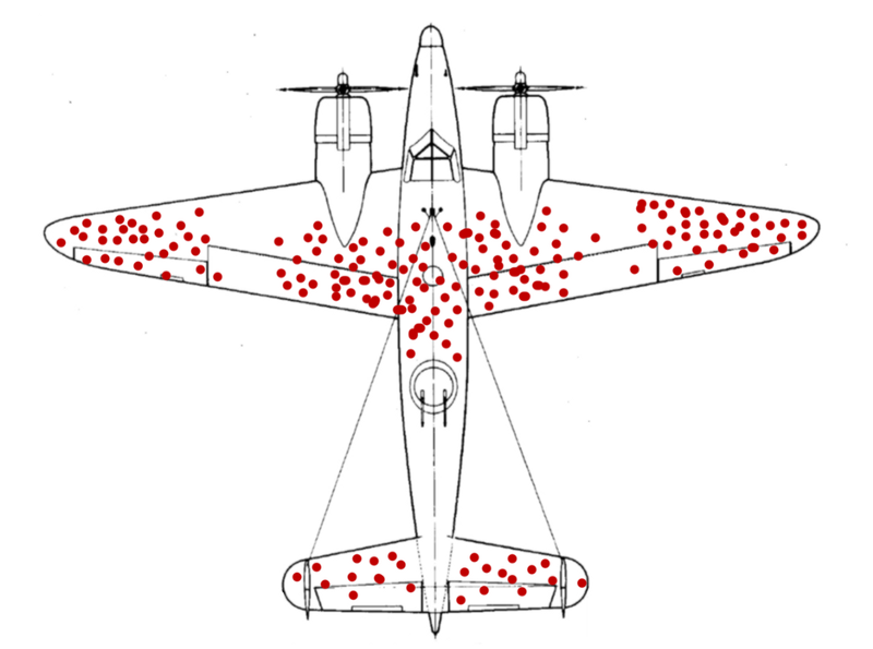
You will notice that most of the damage seems to be in the wings and in the middle of the fuselage (body), while there is little damage to the nose, engines, and back of the fuselage. You might think that means that the wings and middle fuselage are the areas that should be reinforced.
Wald’s team realized that this was wrong: the damage data was collected from planes that returned, which is not a random sample of planes that went out. Planes were probably shot in the nose, the engines, and the back of the fuselage just as often as anywhere else, but they did not appear often in the data because they crashed. Wald’s insight led to a counter-intuitive policy recommendation: reinforce the parts of the plane that usually show the least damage.
There are two basic solutions to missing data:
- Reinterpretation: we redefine the population so that our data
can be correctly interpreted as a random sample from that population.
- Abraham Wald’s team made a distinction between a random sample of planes that flew, and a random sample of planes that returned.
- Canadian survey data can be interpreted as a a random sample of Canadians who answer surveys.
- Imputation: we assume or impute values for all missing quantities.
- Abraham Wald’s team used its domain knowledge to assume that the distribution of damage was roughly uniform across all planes that flew.
- We might assume that Canadians who do not respond to surveys would give similar responses to those given by survey respondents.
- We might assume that Canadians who do not respond to surveys would give similar responses to those given by survey respondents of the same age, gender, and education.
Like many real-world statistical issues, nonresponse and censoring do not have a purely technical solution. Careful thought and domain knowledge are both required. If we are imputing values, do we believe that our imputation method is reasonable? If we are redefining the population, is the redefined population one we care about? There are no clearly right answers to these questions, and sometimes our data are simply not good enough to answer our questions.
Nonresponse bias in US presidential elections
Going into both the 2016 and 2020 US presidential elections, polls indicated that the Democratic candidate had a substantial lead over the Republican candidate:
- Hillary Clinton led Donald Trump by 4-6% nationally in 2016
- Joe Biden led Trump by 8% nationally in 2020.
The actual vote was much closer:
- Clinton won the popular vote (but lost the election) by 2%
- Biden won the popular vote (and won the election) by about 4.5%.
The generally accepted explanation among pollsters for the clear disparity between polls and voting is systematic nonresponse: for some reason, Trump voters are less likely to respond to polls. Since most people do not respond to standard telephone polls any more (response rates are typically around 9%), it does not take much difference in response rates to produce a large difference in responses. For example, suppose that:
- We call 1,000 voters
- These voters are equally split, with 500 supporting Biden and 500 supporting Trump.
- 10% of Biden voters respond (50 voters)
- 8% of Trump voters respond (40 voters)
The overall response rate is \(90/1000 = 9\%\) (similar to what we usually see in surveys), Biden has the support of \(50/90 = 56\%\) of the respondents while Trump has the support of \(40/90 = 44\%\). Actual support is even, but the polls show a 12 percentage point gap in support, entirely because of the small difference in response rates.
Polling organizations employ statisticians who are well aware of this problem, and they made various adjustments after the 2016 election to address it. For example, most now weight their analysis by education, since more educated people tend to have a higher response rate. Unfortunately, the 2020 results indicate that this adjustment was not enough to produce accurate predictions, and the 2024 results faced similar problems.
Chapter review
Statistics is the core subject of this course, making this chapter the most important one in the entire book.
In this chapter we have learned to model a data generating process, describe the probability distribution of a statistic, and interpret a statistic as estimating some unknown parameter of the underlying data generating process.
An estimator is rarely identical to the parameter of interest, so any conclusions based on estimating a parameter of interest have a degree of uncertainty. To describe this uncertainty in a rigorous and quantitative manner, we will next learn some principles of statistical inference.
Practice problems
Answers can be found in the appendix.
GOAL #1: Describe the joint probability distribution of a very simple data set
- Suppose we have a data set \(D_n = (x_1,x_2)\) that is a random sample
of size \(n = 2\) on the random variable \(x_i\) which has discrete PDF:
\[\begin{align}
f_x(a) &= \begin{cases}
0.4 & a = 1 \\
0.6 & a = 2 \\
\end{cases}
\end{align}\]
Let \(f_{D_n}(a,b) = \Pr(x_1=a \cap x_2 = b)\) be the joint PDF of the data set
- Find the support \(S_{D_n}\).
- Find \(f_{D_n}(1,1)\).
- Find \(f_{D_n}(2,1)\).
- Find \(f_{D_n}(1,2)\).
- Find \(f_{D_n}(2,2)\).
GOAL #2: Identify the key features of a random sample
- Suppose we have a data set \(D_n = (x_1,x_2)\) of size \(n = 2\). For
each of the following conditions, identify whether it implies
that \(D_n\) is (i) definitely a random sample; (ii) definitely
not a random sample; or (iii) possibly a random sample.
- The two observations are independent and have the same mean \(E(x_1) = E(x_2) = \mu_x\).
- The two observations are independent and have the same mean \(E(x_1) = E(x_2) = \mu_x\) and variance \(var(x_1)=var(x_2)=\sigma_x^2\).
- The two observations are independent and have different means \(E(x_1) \neq E(x_2)\).
- The two observations have the same PDFs, and are independent.
- The two observations have the same PDFs, and have \(corr(x_1,x_2) = 0\)
- The two observations have the same PDFs, and have \(cov(x_1,x_2) > 0\).
GOAL #3: Classify data sets by sampling types
- Identify the sampling type (random sample, time series, stratified sample,
cluster sample, census, convenience sample) for each of the following data
sets.
- A data set from a survey of 100 SFU students who I found waiting in line at Tim Horton’s.
- A data set from a survey of 1,000 randomly selected SFU students.
- A data set from a survey of 100 randomly selected SFU students from each faculty.
- A data set that reports total SFU enrollment for each year from 2005-2020.
- A data set from administrative sources that describes demographic information and postal code of residence for all SFU students in 2020.
GOAL #4: Find the sampling distribution of a very simple statistic
- Suppose we have the data set described in question 1 above. Find the support
\(S\) and sampling distribution \(f(\cdot)\) for:
- The sample frequency \(\hat{f}_1 = \frac{I(x_1=1) + I(x_2=1)}{2}\).
- The sample average \(\bar{x} = (x_1 + x_2)/2\).
- The sample variance \(sd_x^2 = (x_1-\bar{x})^2 + (x_2-\bar{x})^2\).
- The sample standard deviation \(sd_x = \sqrt{sd_x^2}\).
- The sample minimum \(xmin = \min(x_1, x_2)\).
- The sample maximum \(xmax = \max(x_1, x_2)\).
GOAL #5: Find the mean and variance of a statistic from its sampling distribution
- Suppose we have the data set described in question 1 above. Find the
expected value of:
- The sample frequency \(\hat{f}_1 = \frac{I(x_1=1) + I(x_2=1)}{2}\).
- The sample average \(\bar{x} = (x_1 + x_2)/2\).
- The sample variance \(sd_x^2 = (x_1-\bar{x})^2 + (x_2-\bar{x})^2\).
- The sample standard deviation \(sd_x = \sqrt{sd_x^2}\).
- The sample minimum \(xmin = \min(x_1, x_2)\).
- The sample maximum \(xmax = \max(x_1, x_2)\).
- Suppose we have the data set described in question 1 above. Find the
variance of:
- The sample frequency \(\hat{f}_1 = \frac{I(x_1=1) + I(x_2=1)}{2}\).
- The sample average \(\bar{x} = (x_1 + x_2)/2\).
- The sample minimum \(xmin = \min(x_1, x_2)\).
- The sample maximum \(xmax = \max(x_1, x_2)\).
GOAL #6: Find the mean and variance of a statistic that is linear in the data
- Suppose we have a data set \(D_n = (x_1,x_2)\) that is a random sample
of size \(n = 2\) on the random variable \(x_i\) which has mean \(E(x_i) = 1.6\)
and variance \(var(x_i) = 0.24\). Find the mean and variance of:
- The first observation \(x_1\).
- The sample average \(\bar{x} = (x_1 + x_2)/2\).
- The weighted average \(w = 0.2*x_1 + 0.8*x_2\).
GOAL #7: Distinguish between parameters, statistics, and estimators
- Suppose \(D_n\) is a random sample of size \(n=100\) on a random variable
\(x_i\) which has the \(N(\mu,\sigma^2)\) distribution. Which of the following
are unknown parameters of the DGP? Which are statistics calculated from the
data?
- \(D_n\)
- \(n\)
- \(x_i\)
- \(i\)
- \(N\)
- \(\mu\)
- \(\sigma^2\)
- \(E(x_i)\)
- \(E(x_i^3)\)
- \(var(x_i)\)
- \(sd(x_i)/\sqrt{n}\)
- \(\bar{x}\)
- Suppose we have the data set described in question 1 above. Find the true
value of:
- The probability \(\Pr(x_i=1)\).
- The population mean \(E(x_i)\).
- The population variance \(var(x_i)\).
- The population standard deviation \(sd(x_i)\).
- The population minimum \(\min(S_x)\).
- The population maximum \(\max(S_x)\).
GOAL #8: Calculate the sampling error of an estimator
- Suppose we have the data set described in question 1 above. Suppose we use
the sample maximum \(xmax = \max(x_1,x_2)\) to estimate the population maximum
\(\max(S_x)\).
- Find the support \(S_{err}\) of the sampling error \(err = \max(x_1,x_2) - max(S_x)\).
- Find the PDF \(f_{err}(\cdot)\) for the sampling distribution of the sampling error \(err\).
GOAL #9: Calculate bias and classify estimators as biased or unbiased
Suppose we have the data set described in question 1 above. Classify each of the following estimators as biased or unbiased, and calculate the bias:
- The sample frequency \(\hat{f}_1\) as an estimator of the probability \(\Pr(x_i=1)\).
- The sample average \(\bar{x}\) as an estimator of the population mean \(E(x_i)\)
- The sample variance \(sd_x^2\) as an estimator of the population variance \(var(x_i)\)
- The sample standard deviation \(sd_x\) as an estimator of the population standard deviation \(sd(x_i)\)
- The sample minimum \(xmin\) as an estimator of the population minimum \(\min(S_x)\).
- The sample maximum \(xmax\) as an estimator of the population maximum \(\max(S_x)\).
Suppose we are interested in the following parameters:
- The average earnings of Canadian men: \(\mu_M\).
- The average earnings of Canadian women: \(\mu_W\).
- The male-female earnings gap in Canada: \(\mu_M - \mu_W\).
- The male-female earnings ratio in Canada: \(\mu_M/\mu_W\).
and we have calculated the following statistics from a random sample of Canadians:
- The average earnings of men in our sample \(\bar{y}_{M}\).
- The average earnings of women in our sample \(\bar{y}_{W}\).
- The male-female earnings gap in our sample \(\bar{y}_{M} - \bar{y}_{W}\).
- The male-female earnings ratio in our sample \(\bar{y}_{M}/\bar{y}_{W}\).
We already know that \(\bar{y}_{M}\) is an unbiased estimator of \(\mu_M\) and \(\bar{y}_{W}\) is an unbiased estimator of \(\mu_W\).
- Is the sample earnings gap \(\bar{y}_M - \bar{y}_W\) a biased or unbiased estimator of the population gap \(\mu_M - \mu_W\)? Explain.
- Is the sample earnings ratio \(\bar{y}_M/\bar{y}_W\) a biased or unbiased estimator of the population earnings ratio \(\mu_M/\mu_W\)? Explain.
GOAL #10: Calculate the mean squared error of an estimator
- Suppose we have the data set described in question 1 above. Calculate the
mean squared error for:
- The sample frequency \(\hat{f}_1\) as an estimator of the probability \(\Pr(x_i=1)\).
- The sample average \(\bar{x}\) as an estimator of the population mean \(E(x_i)\).
- The sample minimum \(xmin\) as an estimator of the population minimum \(\min(S_x)\).
- The sample maximum \(xmax\) as an estimator of the population maximum \(\max(S_x)\).
GOAL #11: Apply MVUE and MSE criteria to select an estimator
- Suppose you have a random sample of size \(n=2\) on the random variable
\(x\) with mean \(E\left(x\right)=\mu\) and variance \(var(x_i)=\sigma^2\). Two
potential estimators of \(\mu\) are the sample average:
\[\begin{align}
\bar{x} = \frac{x_1 + x_2}{2}
\end{align}\]
and the last observation:
\[\begin{align}
x_2
\end{align}\]
- Are these estimators biased or unbiased?
- Find \(var(\bar{x})\).
- Find \(var(x_2)\).
- Find \(MSE(\bar{x})\).
- Find \(MSE(x_2)\).
- Which estimator is preferred under the MVUE criterion?
- Which estimator is preferred under the MSE criterion?
GOAL #12: Calculate the standard error for a sample average
- Suppose that we have a random sample \(D_n\) of size \(n=100\) on the random variable \(x_i\) with unknown mean \(\mu\) and unknown variance \(\sigma^2\). Suppose that the sample average is \(\bar{x} = 12\) and the sample variance is \(sd^2 = 4\). Find the standard error of \(\bar{x}\).
GOAL #13: Explain the law of large numbers and what it means for an estimator to be consistent
- Suppose we have a random sample of size \(n\) on the random variable \(x_i\)
with mean \(E(x_i) = \mu\). Which of the following statistics are consistent
estimators of \(\mu\)?
- The sample average \(\bar{x}\)
- The sample median.
- The first observation \(x_1\).
- The average of all even-numbered observations.
- The average of the first 100 observations.
It might be more accurate to say it involves only three unknown probabilities. Since we know the probabilities will sum up to one, if we know three of the four we can calculate the fourth.↩︎
As a technical matter, the assumption of independence requires that we sample with replacement. This means we allow for the possibility that we sample the same case more than once. In practice this doesn’t matter as long as the sample is small relative to the population.↩︎
All random variables we will see in this course will have an expected value, but it is possible for a random variable to have a well-defined PDF but not a well-defined expected value. For example, if \(x \sim N(0,1)\), then \(y=1/x\) has this property.↩︎
Martin Grandjean (vector), McGeddon (picture), Cameron Moll (concept), CC BY-SA 4.0; https://creativecommons.org/licenses/by-sa/4.0/deed.en;, via Wikimedia Commons, https://commons.wikimedia.org/wiki/File:Survivorship-bias.svg.↩︎