Chapter 8 Statistical inference

We can use statistics to describe a data set and to estimate the value of some unknown parameter. But our data typically provide limited evidence on the true value of any parameter of interest: estimates are subject to sampling error of an unknown direction and magnitude. We want to have a way of accounting for sampling error and assessing how strong the evidence is in favor or opposition to a particular claim about the true state of the world.

This chapter will develop a set of techniques for statistical inference: instead of providing a single best guess of a parameter’s true value, we will use data to classify particular parameter values as plausible (could be the true value) or implausible (unlikely to be the true value).

Chapter goals

In this chapter, we will learn how to:

1. Select a parameter of interest, null hypothesis, and alternative hypothesis for a hypothesis test.
2. Identify the characteristics of a valid test statistic.
3. Describe the distribution of a simple test statistic under the null and alternative.
4. Find the size/significance of a simple test.
5. Find critical values for a test of a given size.
6. Implement and interpret a hypothesis test.
7. Construct and interpret a confidence interval.

To prepare for this chapter, please review the chapter on statistics.

8.1 Questions and evidence

We often analyze data with a specific research question in mind. That is, there is some statement about the world whose truth we are interested in assessing. For example, we might want to know:

• Do men earn more than women with similar skills?
• Does increasing the minimum wage reduce employment?
• Do poor economies grow faster or slower than rich ones?

Sometimes the data allow us to answer these questions decisively, sometimes not. That is, the strength of our evidence can vary. The aim of statistical inference is to give us a clear and rigorous way of thinking about the strength of evidence, and a systematic way of setting a standard of evidence for reaching a particular conclusion.

Example 8.1 Fair and unfair roulette games

Suppose you work as a casino regulator for the BCLC (British Columbia Lottery Corporation, the crown corporation that regulates all commercial gambling in B.C.). You have been given data with recent roulette results from a particular casino and are tasked with determining whether the casino is running a fair game.

Before getting caught up in math, let’s think about how we might assess evidence:

1. A fair game implies a particular win probability for each bet.
   • For example, the win probability for a bet on red will be $18/37 \approx 0.486$ in a fair game.
2. The Law of Large Numbers implies that the win rate over many games will be close to the win probability, but the win rate and win probability are unlikely to be identical in a finite sample.
   • In 100 games, we would expect red to win about 48 or 49 times in a fair game.
   • But these are games of chance; even in a fair game, red may win a little more or less than expected.
3. In a given data set:
   • We might have results from many games, or only a few games.
   • Our results may have a win rate close to the expected rate for a fair game, or far from that rate.

We can put those possibilities into a table, and make an assessment of what we might conclude from a given data set:

Observed win rate	Many games	Just a few games
Close to $48.6\%$	Probably fair	Could be fair or unfair
Far from $48.6\%$	Probably unfair	Could be fair or unfair

That is, we can make a fairly confident conclusion if we have a lot of evidence, and our conclusion depends on what the evidence shows. But if we do not have a lot of evidence, we cannot make a confident conclusion either way.

This chapter will formalize these basic ideas about evidence.

8.2 Hypothesis tests

We will start with hypothesis tests. The idea of a hypothesis test is to determine whether the data rule out or reject a specific value of the unknown parameter of interest $\theta$.

A hypothesis test consists of the following components:

1. A null hypothesis $H_0$ and alternative hypothesis $H_1$ about the parameter of interest $\theta$.
2. A test statistic $t_n$ that can be calculated from the data.
3. A pair of critical values $c_L$ and $c_H$, such that the null hypothesis will be rejected if $t_n$ is not between $c_L$ and $c_H$.

We will go through each of these components in detail.

8.2.1 Data and DGP

For the remainder of this chapter, suppose we have a data set $D_n$ of size $n$. The data comes from an unknown data generating process $f_D$.

Example 8.2 Data and DGP for roulette

Let $D_n = (x_1,\ldots,x_n)$ be a data set of results from $n = 100$ games of roulette at a local casino. More specifically,let: $$\begin{align} x_i = I(\textrm{Red wins}) \end{align}$$ We will consider two cases:

Case number	Wins by red (out of 100)	$\bar{x}$	$sd_x$
$1$	$35$	$0.35$	$0.479$
$2$	$40$	$0.40$	$0.492$

In both cases, red wins somewhat less than we would expect in a fair game. This could be just a fluke, or it could be a sign that the game is unfair.

8.2.2 The null and alternative hypotheses

The first step in a hypothesis test is to identify the parameter of interest and define the null hypothesis. The null hypothesis is a statement about the parameter of interest $\theta$ that takes the form: $$\begin{align} H_0: \theta = \theta_0 \end{align}$$ where $\theta = \theta(f_D)$ is the parameter of interest and $\theta_0$ is a specific value we are interested in ruling out.

The next step is to define the alternative hypothesis, which is every other value of $\theta$ we are willing to consider. In this course, the alternative hypothesis will always be: $$\begin{align} H_1: \theta \neq \theta_0 \end{align}$$ where $\theta_0$ is the same number as used in the null.

Example 8.3 Null and alternative for roulette

In our roulette example, the parameter of interest is the win probability for red: $$\begin{align} p_{red} = \Pr(x_i = 1) \end{align}$$ The null hypothesis is that the game is fair: $$\begin{align} H_0: p_{red} = 18/37 \end{align}$$ and the alternative hypothesis is that it is not fair: $$\begin{align} H_1: p_{red} \neq 18/37 \end{align}$$ I am expressing the fair win probability as a fraction to minimize rounding error in subsequent calculations.

What null hypothesis to choose?

Our framework here assumes that you already know what null hypothesis you wish to test, but we might briefly consider how we might choose a null hypothesis to test.

In some applications, the research question leads to a natural null hypothesis:

• The natural null in our roulette example is to test is whether the win probability matches that of a fair game ($p = 18/37$).
• When measuring the effect of one variable on another, the natural null to test is “no effect at all” ($\theta = 0$).
• In epidemiology, a contagious disease will tend to spread if its reproduction rate $R$ is greater than one, and decline if it is less than one, so the natural null to test is $R = 1$.

If there is no obvious null hypothesis, it may make sense to test many null hypotheses and report all of the results.

8.2.3 The test statistic

Our next step is to construct a test statistic that can be calculated from our data. A valid test statistic for a given null hypothesis is a statistic $t_n$ that has the following two properties:

1. The probability distribution of $t_n$ under the null (i.e., when $H_0$ is true) is known.
2. The probability distribution of $t_n$ under the alternative (i.e., when $H_1$ is true) is different from its probability distribution under the null.

It is not easy to come up with a valid test statistic, so that is typically a job for a professional statistician. But I want you to understand the basic idea of what a test statistic is, and to be able to tell whether a proposed test statistic is valid or not.

Example 8.4 A test statistic for roulette

A natural test statistic for determining whether the game is fair is the number of wins for red: $$\begin{align} t_n = n\hat{f}_{red} = n\bar{x}_n =\sum_{i=1}^n x_i \end{align}$$ Since a fair game has win probability $18/37 \approx 0.486$ we would expect about 48 or 49 wins in 100 fair games.

Once we have a proposed test statistic, we need to find its probability distribution under the null. Remember, this needs to be a specific probability distribution with no unknown parameters.

Example 8.5 The distribution under the null

We earlier learned about the binomial distribution, which is the distribution of the number of times an event with probability $p$ happens in $n$ independent trials. Since each $x_i$ in our data is an independent $Bernoulli(p_{red})$ random variable, the number of wins is binomial: $$\begin{align} t_n \sim Binomial(100,p_{red}) \end{align}$$

Under the null (when $H_0$ is true), $p_{red} = 18/37$ and so: $$\begin{align} H_0 \quad \implies \qquad t_n \sim Binomial(100,18/37) \end{align}$$ Since this distribution does not involve any unknown parameters, our test statistic satisfies the requirement of having a known distribution under the null.

The next step is to describe the probability distribution of the test statistic under the alternative. It’s OK if this distribution includes unknown parameters, the key is to confirm that it is different from the distribution under the null.

Example 8.6 The distribution under the alternative

Under the alternative (when $H_1$ is true), $p_{red}$ can take on any value other than $18/37$. The sample size is still $n=100$, so the distribution of the test statistic is: $$\begin{align} H_1 \quad \implies \qquad t_n \sim Binomial(100,p_{red}) \textrm{ where $p_{red} \neq 18/37$ } \end{align}$$ Notice that the distribution of our test statistic under the alternative is not known, since $p_{red}$ is not known. But the distribution is different under the alternative, and that is what we require from our test statistic.

8.2.4 Size and power

After choosing a test statistic $t_n$ and determining its distribution under the null, the next step is to choose critical values. The critical values of a test are two numbers $c_L$ and $c_H$ (where $c_L < c_H$) such that:

1. $t_n$ has a high probability of being between $c_L$ and $c_H$ when the null is true.
2. $t_n$ has a lower probability of being between $c_L$ and $c_H$ when the alternative is true.

The range of values from $c_L$ to $c_H$ is called the critical range of our test.

Given the test statistic and critical values:

• We reject the null if $t_n$ is outside of the critical range.
  • This means we have clear evidence that $H_0$ is false.
  • The reason we reject here is that we know we would be unlikely to observe such a value of $t_n$ if $H_0$ were true.
• We fail to reject the null or accept the null if $t_n$ is inside of the critical range.
  • This means we do not have clear evidence that $H_0$ is false.
  • This does not mean we have clear evidence that $H_0$ is true. We may just not have enough evidence to tell whether it is true or false.
  • I usually avoid saying “accept the null” because it can be misleading.

We reject the null if the test statistic falls outside of the blue critical range above

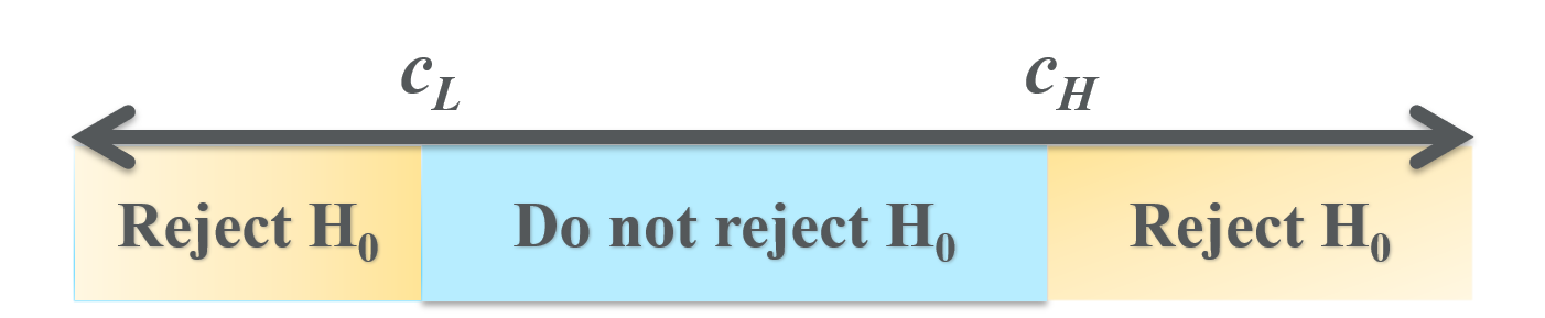
Example 8.7 Proposed critical values for the win frequency

Suppose we pick the following critical values for our test: $$\begin{align} c_L &= 45 \\ c_H &= 55 \end{align}$$ This means:

• We reject the null of a fair game if red wins fewer than 45 games $(t_n < c_L)$.
• We reject the null of a fair game if red wins more than 55 games $(t_n > c_H)$.

Otherwise, we accept or fail to reject the null of a fair game.

How do we choose critical values? You can think of critical values as setting a standard of evidence, so we need to balance two considerations:

• The probability of rejecting a false null is called the power of the test.
  • We want to reject false nulls, so power is good.
• The probability of rejecting a true null is called the size or significance of a test.
  • We do not want to reject true nulls, so size is bad.

The size of a test is a number: $$\begin{align} size &= \Pr(\textrm{reject $H_0$}) \qquad \textrm{when $H_0$ is true} \end{align}$$ and it is usually easy to calculate.

Example 8.8 The size of our proposed test

With our proposed critical values $(c_L,c_H) = (45,55)$, we can calculate the size of our test by following these steps:

1. Find the probability of rejecting the null as a function of the (potentially unknown) CDF of the test statistic: $$\begin{align} \Pr(\textrm{reject $H_0$}) &= \Pr((t_n < 45) \cup (t_n > 55)) \\ &= \Pr(t_n < 45) + \Pr(t_n > 55) \\ &= \Pr(t_n \leq 44) + (1 - \Pr(t_n \leq 55)) \\ &= F_t(44) + (1 - F_t(55)) \end{align}$$ where $F_t(\cdot)$ is the CDF of $t_n$.

2. Find the CDF under the null and substitute: When the null is true, we know that: $$\begin{align} H_0 &\implies t_n \sim Binomial(100,18/37) \end{align}$$ and we can calculate this CDF in Excel using the BINOM.DIST() function. The correct formula for $F_t(44)$ is =BINOM.DIST(44,100,18/37,TRUE) and the formula for $F_t(55)$ is =BINOM.DIST(55,100,18/37,TRUE) which produces: $$\begin{align} \Pr(\textrm{reject $H_0$}) &= F_t(44) + (1 - F_t(55)) \\ &\approx 0.20 + (1 - 0.91)) \\ &\approx 0.29 \end{align}$$ In R, the function for the binomial CDF is pbinom() and the code would be:

   pbinom(44, 100, 18/37) + 1 - pbinom(55, 100, 18/37)
   ## [1] 0.2885956

So the size of this test is about 29%. That is, if the game is fair we have a 29% chance of mistakenly concluding it is unfair. This is a pretty high probability, suggesting we might need to choose different critical values.

The power of a test is a function: $$\begin{align} power(\theta) &= \Pr(\textrm{reject $H_0$}) \qquad \textrm{when $H_0$ is false} \end{align}$$ and is more difficult to calculate.

Example 8.9 The power of our proposed test

With our proposed critical values $(c_L,c_H) = (45,55)$, we can also find the power of our test by following these steps:

1. Find the probability of rejecting the null as a function of the (potentially unknown) CDF of the test statistic. We already did this: $$\begin{align} \Pr(\textrm{reject $H_0$}) &= F_t(44) + (1 - F_t(55)) \end{align}$$ where $F_t(\cdot)$ is the CDF of $t_n$.

2. Pick a parameter value for which you wish to calculate power. For example, let’s pick $p_{red}=0.4$.

3. Find the CDF for the chosen parameter value and substitute. In general, $$\begin{align} H_1 &\implies t_n \sim Binomial(100,p_{red}) \qquad \textrm{where $p_{red} \neq 18/37$} \end{align}$$ and for our chosen parameter value $p_{red}=0.4$ $$\begin{align} p_{red}=0.4 &\implies t_n \sim Binomial(100,0.4) \end{align}$$ We can calculate these probabilities in Excel using the =BINOM.DIST() function. The formula for $F_t(44)$ is =BINOM.DIST(44,100,0.4,TRUE) and the formula for $F_t(55)$ is =BINOM.DIST(55,100,0.4,TRUE) which produces: $$\begin{align} power(0.4) &= \Pr(\textrm{reject $H_0$}) \\ &= F_t(44) + (1 - F_t(55)) \\ &\approx 0.821 + (1 - 0.999)) \\ &\approx 0.822 \end{align}$$ In R, the code would be:

   pbinom(44, 100, 0.4) + 1 - pbinom(55, 100, 0.4)
   ## [1] 0.8219802

That is, if the true win probability is 40%, the probability of rejecting the null of a fair game is about 82%.

We can calculate $power(\theta)$ for many values of $\theta$ and plot the result to get what is called a power curve. Creating power curves is sometimes complex, and is beyond the scope of this course. But we can at least view and interpret a power curve.

Example 8.10 A power curve for our proposed test

We can calculate the power for any value of $p$ and plot the result as a power curve: Most power curves look like Figure 8.1 below: power is low for values close to the null, and rises as we get further from the null. Power is a probability, so it never goes above one or below zero.

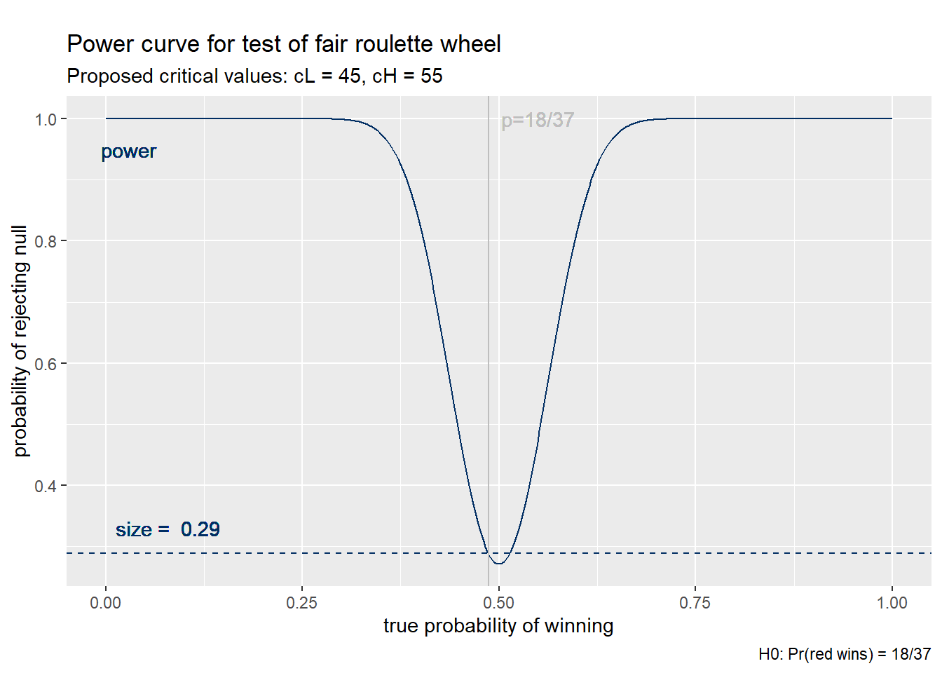
Figure 8.1: Power curve for proposed critical values

When choosing critical values, there is always a trade off between power and size:

• A wider critical range (lower $c_L$ or higher $c_H$) is more conservative:
  • It produces fewer rejections.
  • It has low power (bad).
  • It has low size (good).
• A narrower critical range (higher $c_L$ or lower $c_H$) is more aggressive:
  • Produces more rejections.
  • Has greater power (good).
  • Has greater size (bad).

The appropriate critical range depends on how we view this trade off: are we more concerned about the risk of rejecting a true null, or failing to reject a false null?

Example 8.11 Power and size for other critical values

If we use a wider critical range $(c_L,c_H) = (40,60)$, we can follow the same calculations as in the previous examples to find: $$\begin{align} size &\approx 0.042 \\ power(0.4) &\approx 0.462 \end{align}$$ Using this wider critical range substantially reduces the probability of mistakenly rejecting a true null (from 29% to 4%) but this comes at a cost of reducing the probability of rejecting the null when it is false (e.g., from 82% to 46% when $p=0.4$).

Figure 8.2 shows the full power curve for this critical range. As the figure shows, the wider critical range has lower size, but at a cost of lower power for every value of the win probability.

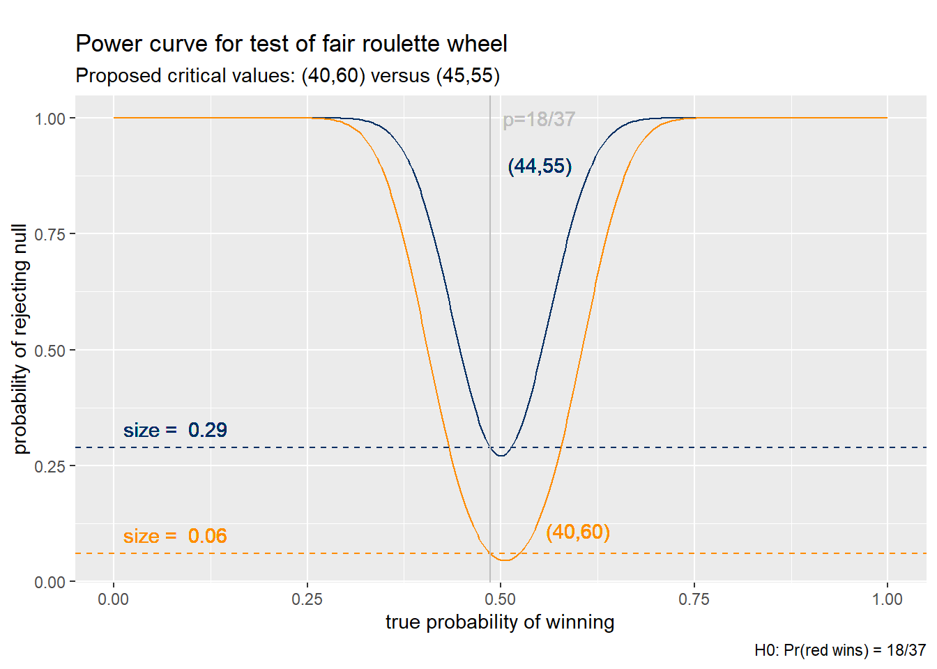
Figure 8.2: Power curve comparison

8.2.5 Choosing critical values

Given the trade off between power and size, we could construct some criterion that accounts for both (just like MSE includes both variance and bias) and choose critical values to maximize that criterion. But we don’t do that, in part because power is tough to calculate.

Instead, we follow a simple convention:

1. Set the size to a fixed value $\alpha$.
   • The convention in economics and most other social sciences is to use a size of 5% ($\alpha = 0.05$).
   • Economists may use 1% ($\alpha = 0.01$) when working with larger data sets or 10% ($\alpha = 0.10$) when working with smaller data sets.
   • The data sets in physics or genetics are much larger, and their convention is to use a much lower size.
2. Find critical values that imply the desired size.
   • With a size of 5% $(\alpha = 0.05)$, we would:
     • Set $c_L$ to the 2.5 percentile (0.025 quantile) of the null distribution.
     • Set $c_H$ to the 97.5 percentile (0.975 quantile) of the null distribution.
   • With a size of 10% $(\alpha = 0.10)$, we would:
     • Set $c_L$ to the 5 percentile (0.05 quantile) of the null distribution.
     • Set $c_H$ to the 95 percentile (0.95 quantile) of the null distribution.
   • More generally, with a size of $\alpha$, we would:
     • Set $c_L$ to the $\alpha/2$ quantile of the null distribution.
     • Set $c_H$ to the $1-\alpha/2$ quantile of the null distribution.

Note that we are dividing the size by two so we can put half on the lower tail of the null distribution and half on the upper tail.

Example 8.12 5% critical values for roulette

We earlier showed that the distribution of $t_n$ under the null is: $$\begin{align} t_n \sim Binomial(100,18/37) \end{align}$$ We can get a size of 5% by choosing: $$\begin{align} c_L &= 2.5 \textrm{ percentile of } Binomial(100,18/37) \\ c_H &= 97.5 \textrm{ percentile of } Binomial(100,18/37) \end{align}$$ We can then use Excel or R to calculate these critical values. In Excel, the function you would use is BINOM.INV()

• The formula to calculate $c_L$ is =BINOM.INV(100,18/37,0.025)
• The formula to calculate $c_H$ is =BINOM.INV(100,18/37,0.975)

In R, the function would be qbinom() and the code would be:

cat("2.5 percentile of binomial(100,18/37) =", qbinom(0.025, 100, 18/37), "\n")
## 2.5 percentile of binomial(100,18/37) = 39
cat("97.5 percentile of binomial(100,18/37) =", qbinom(0.975, 100, 18/37), "\n")
## 97.5 percentile of binomial(100,18/37) = 58

In other words we reject the null (at 5% significance) that the roulette wheel is fair if red wins fewer than 39 games or more than 58 games.

P values

The convention of always using a 5% significance level for hypothesis tests is somewhat arbitrary and has some negative unintended consequences:

1. Sometimes a test statistic falls just below or just above the critical value, and small changes in the analysis can change a result from reject to cannot-reject.
2. In many fields, unsophisticated researchers and journal editors misinterpret “cannot reject the null” as “the null is true.”

One common response to these issues is to report what is called the p-value of a test. The p-value of a test is defined as the significance level at which one would switch from rejecting to not-rejecting the null. For example:

• If the p-value is 0.43 (43%) we would not reject the null at 10%, 5%, or 1%.
• If the p-value is 0.06 (6%) we would reject the null at 10% but not at 5% or 1%.
• If the p-value is 0.02 (2%) we would reject the null at 10% and 5% but not at 1%.
• If the p-value is 0.001 (0.1%) we would reject the null at 10%, 5%, and 1%.

The p-value of a test is simple to calculate from the test statistic and its distribution under the null. I won’t go through that calculation here.

8.2.6 Increasing power

Since critical values are set to achieve a fixed size, the only way to increase power is by collecting more data.

Example 8.13 The power curve for the 5% test

Figure 8.3 below depicts the power curve for the 5% test we have just constructed; that is, we are testing the null that $p_{red} = 18/37$ at a 5% size. The blue line depicts the power curve for $n=100$ as in our example, while the orange line depicts the power curve for a smaller sample of size $n=20$ and the purple line depicts the power curve for a larger sample size of size $n=300$. There are a few features I would like you to notice, all of which are common to most regularly used tests:

• Power reaches its lowest value near¹² the point $(18/37,0.05)$. Note that $18/37$ is the parameter value under the null, and $0.05$ is the size of the test. In other words:
  • The power of this test is typically greater than its size.
  • We are more likely to reject the null when it is false than when it is true.
  • A test has this desirable property is called an unbiased test.
• Power increases as the true $p_{red}$ gets further from the null.
  • We are more likely to detect unfairness in a game that is very unfair than when in one that is a little unfair.
• Power also increases with the sample size;
  • The purple line ($n = 300$) is above the blue line ($n = 100$), which is above the orange line ($n = 20$).
  • As $n \rightarrow \infty$, power goes to one for every value in the alternative. A test with this desirable property is called a consistent test. You can ignore the dashed lines for the moment.

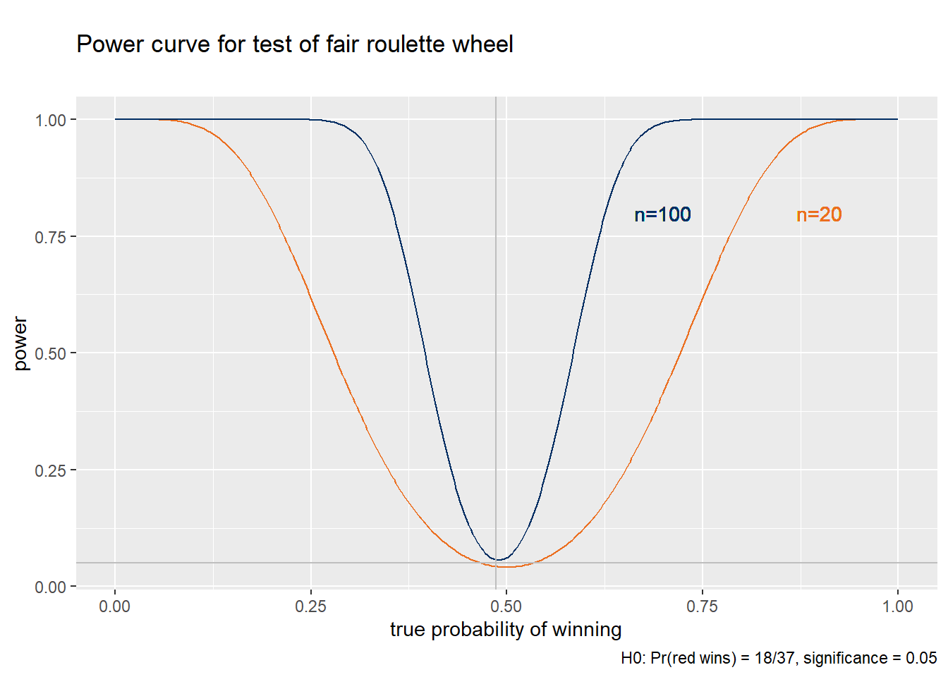
Figure 8.3: Power curves for the roulette example

Power analysis is often used by researchers to determine how much data to collect. Each additional observation collected increases power without increasing size, but each additional observation costs money. With limited research funding, it is important to spend enough to get clear results, but not much more than that.

Example 8.14 How many observations do we need?

We can use the power curve to decide how much data to collect. For example, we might ask “how many observations do I need to have an 80% chance of rejecting the null of a fair game $(p = 18/37 \approx 0.486)$ when the true win probability is 40% $(p = 0.4)$?”

In Figure 8.3, this means the power curve would need to be above the point where the two dashed purple lines intersect. This represents the point where $power(0.4) = 0.8$.

• A sample size of 20 is not big enough, as the orange power curve for $n=20$ is below this point.
• A sample size of 100 is not big enough, as the blue power curve for $n=100$ is below this point.
• A sample size of 300 is more than big enough, as the purple power curve for $n=300$ is above this point.

So the minimum sample size needed to achieve our goal of $power(0.4) \geq 0.8$ is somewhere between 100 and 300. I’ve done the calculation, and the precise number is 251.

8.2.7 Implementation

The steps taken above derive a test for a specific null hypothesis (a fair roulette game) for a specific sample size (100) and desired significance level (5%). But the results can be generalized to a hypothesis test for any event probability.

Example 8.15 A general test for a single probability

We can generalize the test we have constructed so far to the case of the probability of any event:

Test component	Roulette example	General case
Parameter	$p_{red} = \Pr(\textrm{Red wins})$	$p = \Pr(\textrm{event})$
Null hypothesis	$H_0:p_{red} = 18/37$	$H_0:p = p_0$
Alternative hypothesis	$H_1: p_{red} \neq 18/37$	$H_1: p \neq p_0$
Test statistic	$t = n\hat{f}_{red}$	$t = n\hat{f}_{\textrm{event}}$
Null distribution	$Binomial(100,18/37)$	$Binomial(n,p_0)$
Size/significance	5% (0.05)	$\alpha$
Critical value $c_L$	39	2.5 percentile of $Binomial(n,p_0)$
Critical value $c_H$	58	97.5 percentile of $Binomial(n,p_0)$
Decision	Reject if $t \notin [39,58]$	Reject if $t \notin [c_L,c_H]$

So far, we have discussed how to construct a hypothesis test from scratch. But data analysts mostly use off-the-shelf test statistics and critical values that have been developed by professional statisticians.

The main task of a person working with data is implementing the test and interpreting the results:

1. Choose your null and alternative hypotheses.
   • These depend on your research question, so you must choose them yourself.
2. Choose the desired size of your test.
   • In economics, it is usually 5%.
3. Construct or look up an appropriate test. A test consists of:
   • Your null and alternative hypotheses.
   • A test statistic.
   • Critical values (for your chosen size).
4. Calculate the test statistic based on your data.
5. Compare the test statistic to the critical values and make an accept/reject decision.
6. Interpret your findings.
   • Remember that failing to reject the null does not mean the null is true. It usually means the evidence is inconclusive on whether the null is true.

Example 8.16 Implementing our roulette test

To review the roulette example, the null hypothesis is: $$\begin{align} H_0: p_{red} &= 18/37 \\ H_1: p_{red} &\neq 18/37 \end{align}$$ the test statistic is the absolute win frequency: $$\begin{align} t_n = n\bar{x} \end{align}$$ and we want the test to have 5% significance, which implies critical values of $$\begin{align} c_L &= 39 \\ c_H &= 58 \end{align}$$ We are now ready to implement the test with data. Consider two cases:

Case 1: Red wins in 35 of the 100 games. Do we have a fair game?

• The test statistic is $t_n = 35$, which is outside of the critical range of $[39,58]$.
• We therefore reject the null hypothesis of a fair game.
• That means we have clear evidence that the game is unfair.

Case 2: Red wins in 40 of the 100 games. Do we have a fair game?

• The test statistic is $t_n = 40$, which is inside the critical range of $[39,58]$.
• We therefore fail to reject the null hypothesis of a fair game.
• That means we do not have clear evidence that the game is unfair.

Remember that failing to reject the null does not mean the null is true. It is still possible that the game is unfair, we just don’t have clear evidence that it is. We may need to collect more data to get clearer evidence and increase the power of our test.

8.3 The Central Limit Theorem

In a hypothesis test, the exact probability distribution of the test statistic must be known under the null hypothesis. The example test in the previous section worked because it was based on a sample frequency, a statistic whose probability distribution (binomial) is relatively easy to calculate. Unfortunately, most statistics do not have a probability distribution that is easy to calculate.

Fortunately, we have a very powerful asymptotic result called the Central Limit Theorem (CLT). The CLT roughly says that we can approximate the entire probability distribution of the sample average $\bar{x}_n$ by a normal distribution if the sample size is sufficiently large.

The Central Limit Theorem

As we did with the Law of Large Numbers, we will need to invest in some terminology before we can state the Central Limit Theorem.

Let $s_n$ be a statistic calculated from $D_n$ and let $F_n(\cdot)$ be its CDF. We say that $s_n$ converges in distribution to a random variable $s$ with CDF $F(\cdot)$, or: $$\begin{align} s_n \rightarrow^D s \end{align}$$ if: $$\begin{align} \lim_{n \rightarrow \infty} |F_n(a) - F(a)| = 0 \end{align}$$ for every $a \in \mathbb{R}$.

Convergence in distribution means we can approximate the actual CDF $F_n(\cdot)$ of $s_n$ with its limit $F(\cdot)$. As with most approximations, this is useful whenever $F_n(\cdot)$ is difficult to calculate and $F(\cdot)$ is easy to calculate.

We can now state the theorem:

CENTRAL LIMIT THEOREM: Let $\bar{x}_n$ be the sample average from a random sample of size $n$ on the random variable $x_i$ with mean $E(x_i) = \mu_x$ and variance $var(x_i) = \sigma_x^2$. Let $z_n$ be a standardization of $\bar{x}$: $$\begin{align} z_n = \sqrt{n} \frac{\bar{x} - \mu_x}{\sigma_x} \end{align}$$ Then $z_n \rightarrow^D z \sim N(0,1)$.

Fundamentally, the Central Limit Theorem means that if $n$ is big enough then the probability distribution of $\bar{x}_n$ is approximately normal no matter what the original distribution of $x_i$ looks like.

• In order for the CLT to apply, we need to standardize $\bar{x}_n$ so that it has constant mean (zero) and variance (one) as $n$ increases. That re-scaled sample average is called $z_n$.
• In practice, we don’t usually know $\mu_x$ or $\sigma_x$ so we can’t calculate $z_n$ from data. Fortunately, there are some tricks for getting around this problem that we will talk about later.

What about statistics other than the sample average? Well it turns out that Slutsky’s theorem also extends to convergence in distribution. In combination with the Central Limit Theorem, this means most statistics have an approximately normal distribution if the sample size is big enough.

Slutsky’s theorem for probability distributions

We earlier stated Slutsky’s theorem for convergence in probability, which says that any continuous function of a statistic that converges in probability also converges in probability. We also said that most commonly-used statistics - sample variance and standard deviation, sample frequencies, sample median and quantiles/percentiles, etc. - can be expressed as continuous functions of a set of sample averages. This means that the Law of Large Numbers can be applied to these statistics, which implies that they are all consistent estimators.

There is also a version of Slutsky’s theorem for convergence in distribution:

SLUTSKY THEOREM: Let $g(\cdot)$ be a continuous function. Then: $$\begin{align} s_n \rightarrow^D s \implies g(s_n) \rightarrow^D g(s) \end{align}$$

The implication is that we can extend the Central Limit Theorem to most commonly-used statistics, so these statistics are also asymptotically normal.

8.4 Inference on the mean

Having described the general framework of hypothesis testing and explored a single example in detail, we now move on to the most common application of statistical inference: constructing hypothesis tests and confidence intervals on the mean in a random sample.

Let $D_n = (x_1,\ldots,x_n)$ be a random sample of size $n$ on some random variable $x_i$ with unknown mean $E(x_i) = \mu_x$ and variance $var(x_i) = \sigma_x^2$. Let the sample average be $\bar{x}_n = \frac{1}{n} \sum_{i=1}^n x_i$, let the sample variance be $sd_x^2 = \frac{1}{n-1} \sum_{i=1}^n (x_i - \bar{x})^2$ and let the sample standard deviation be $sd_x = \sqrt{sd_x^2}$.

Example 8.17 The mean and variance in the roulette data

In our roulette data, the random variable $x_i$ has the Bernoulli distribution: $$\begin{align} x_i &\sim Bernoulli(p_{red}) \end{align}$$ where $p_{red}$ is the win probability. We can calculate the mean and variance of $x_i$ directly, or we can look up results for the Bernoulli distribution to get: $$\begin{align} \mu_x &= E(x_i) = p_{red} \\ \sigma_x^2 &= var(x_i) = p_{red} -p_{red}^2 \end{align}$$ so any hypothesis about $p_{red}$ can also be expressed as a hypothesis about $\mu_x$.

Similarly, the sample average is also the win frequency: $$\begin{align} \bar{x}_n &= \frac{1}{n} \sum_{i=1}^{n} x_i = \frac{\textrm{number of wins}}{\textrm{number of games}} \end{align}$$ and we can show that the sample variance can be written: $$\begin{align} sd_x^2 &= \frac{1}{n-1} \sum_{i=1}^{n} (x_i - \bar{x}_n)^2 = \frac{n}{n-1} \left( \bar{x}_n -\bar{x}_n^2 \right) \end{align}$$

Previously, we developed an exact frequency-based test for the fairness of a roulette table. We can also use these results to fit that research question into the mean-based framework of this section.

8.4.1 The null and alternative hypotheses

Suppose that you want to test the null hypothesis: $$\begin{align} H_0: \mu_x = \mu_0 \end{align}$$ against the alternative hypothesis: $$\begin{align} H_1: \mu_x \neq \mu_0 \end{align}$$ where $\mu_0$ is a number that has been chosen to reflect the research question.

Example 8.18 Null and alternative hypotheses for the mean in roulette

The null hypothesis of a fair game can be expressed in terms of $\mu_x$: $$\begin{align} H_0: \mu_x = 18/37 \end{align}$$ against the alternative hypothesis: $$\begin{align} H_1: \mu_x \neq 18/37 \end{align}$$ i.e., $\mu_0 = 18/37$.

8.4.2 The T statistic

Having stated our null and alternative hypotheses, we need to construct a test statistic.

The typical test statistic we use in this setting is called the T statistic, and takes the form: $$\begin{align} t_n = \frac{\bar{x}_n - \mu_0}{sd_x/\sqrt{n}} \end{align}$$ The idea here is that we take our parameter estimate ($\bar{x}_n$), subtract its expected value under the null ($\mu_0$), and divide by its standard error ($sd_x/\sqrt{n}$).

Example 8.19 The T statistic in roulette

Case 1: Red wins in 35 of 100 games, implying that $\bar{x}_n = 0.35$ and $sd_x \approx 0.479$. So the T statistic for our test is: $$\begin{align} t_n &= \frac{\bar{x}_n-\mu_0}{sd_x/\sqrt{n}} \\ &\approx \frac{0.35 - 18/37}{0.479/\sqrt{100}} \\ &\approx -2.84 \end{align}$$

Case 2: Red wins in 40 of the 100 games, implying that $\bar{x}_n = 0.40$ and $sd_x \approx 0.492$. So the T statistic for our test is: $$\begin{align} t_n &= \frac{\bar{x}_n-\mu_0}{sd_x/\sqrt{n}} \\ &\approx \frac{0.40 - 18/37}{0.492/\sqrt{100}} \\ &\approx -1.75 \end{align}$$ Note that the value of $\mu_x$ under the null is $\mu_0=18/37$.

8.4.3 Exact and approximate tests

Next we need to show that this test statistic has a known distribution under the null and a different distribution under the alternative. We can do some algebra to get: $$\begin{align} t_n &= \frac{\bar{x}_n + (\mu_x - \mu_x) - \mu_0}{sd_x/\sqrt{n}} \\ &= \frac{\bar{x}_n - \mu_x}{sd_x/\sqrt{n}} + \frac{\mu_x - \mu_0}{sd_x/\sqrt{n}} \\ &= \frac{\bar{x}_n - \mu_x}{sd_x/\sqrt{n}} \frac{\sigma_x}{\sigma_x} + \frac{\mu_x - \mu_0}{sd_x/\sqrt{n}} \\ &= \underbrace{\frac{\bar{x}_n - \mu_x}{\sigma_x/\sqrt{n}}}_{z_n} \underbrace{\frac{\sigma_x}{sd_x}}_{\textrm{?}} + \underbrace{\sqrt{n} \frac{\mu_x - \mu_0}{sd_x}}_{\textrm{$=0$ if $H_0$ is true}} \end{align}$$ Let’s take a look at the components of this expression:

1. The first term $z_n = \frac{\bar{x}_n - \mu_x}{\sigma_x/\sqrt{n}}$ is a standardization of $\bar{x}_n$. By construction it has the following properties:
   • Mean zero: $E(z_n) = 0$.
   • Unit variance: $var(z_n) = sd(z_n) = 1$.
   • The Central Limit Theorem applies: $z_n \rightarrow^D N(0,1)$.
2. The second term $\frac{\sigma_x}{sd_x}$ features the standard deviation ($\sigma_x$) divided by a consistent estimator of the standard deviation ($sd_x$).
   • In a given sample, this will be almost but not quite equal to one.
3. The third term $\sqrt{n} \frac{\mu_x - \mu_0}{s_x}$ features a positive number that is growing to infinity as the sample size increases ($\sqrt{n}$) times a number that is zero if the null is true and nonzero if the null is false ($\mu_x - \mu_0$), divided by a positive random variable ($s_x$).
   • When the null is true, this term is zero.
   • When the null is false, this term is nonzero and will be large if the sample is large.

Recall that we need the probability distribution of $t_n$ to be known when $H_0$ is true, and different when it is false. The second criterion is clearly met, and the first criterion is met if we can find the probability distribution of $\frac{\bar{x}_n - \mu_x}{sd_x/\sqrt{n}}$.

The frequency-based test we derived in Section 8.2 is what statisticians call an exact test:

1. Exact test: Use the actual finite-sample distribution of the test statistic under the null to derive critical values.

An exact test was possible in this case because the structure of the problem implied that the win count must have a binomial distribution. Unfortunately, an exact test based on the T statistic is only possible if we know the exact probability distribution of $x_i$, and can then use that probability distribution to derive the exact probability distribution of $t_n$.

There are two standard solutions to this problem, both of which are based on approximating an exact test:

2. Parametric test: Assume a specific probability distribution (usually a normal distribution) for $x_i$. We can (or at least a professional statistician can) then mathematically derive the distribution of any test statistic from this distribution.
3. Asymptotic test: Use the Central Limit Theorem to get an approximate probability distribution for the test statistic.

We will explore both of these options. If the distinction between exact, parametric, and asymptotic tests is not clear, read ahead and then come back here.

Example 8.20 An exact test for the T statistic?

With a lot of work, we could derive the exact distribution of the T statistic in our roulette example. This is because we know the exact distribution $x_i \sim Bernoulli(18/37)$ under the null, and could use that information to derive the distribution of any statistic based on $x_i$.

But we won’t do that here, for two reasons:

1. It would be difficult, and we want something easy.
2. The roulette data is a special case, and we want something that will work more generally.

So we will pretend we do not know an exact test is possible, and proceed with approximate tests.

8.4.4 Asymptotic critical values

We will start with the asymptotic solution to the problem. The Central Limit Theorem tells us that: $$\begin{align} \frac{\bar{x}_n - \mu_x}{\sigma_x/\sqrt{n}} \rightarrow^D N(0,1) \end{align}$$ Under the null, our test statistic looks just like this, but with the sample standard deviation $sd_x$ in place of the population standard deviation $\sigma_x$. It turns out that Slutsky’s theorem allows us to make this substitution, and it can be proved that: $$\begin{align} \frac{\bar{x}_n - \mu_x}{sd_x/\sqrt{n}} \rightarrow^D N(0,1) \end{align}$$ Therefore, the null implies that $t_n$ is asymptotically normal: $$\begin{align} (H_0:\mu_x = \mu_0) \qquad \implies \qquad t_n \rightarrow^D N(0,1) \end{align}$$ In other words, we do not know the exact (finite-sample) distribution of $t_n$ under the null, but we know that $N(0,1)$ provides a useful asymptotic approximation to that distribution.

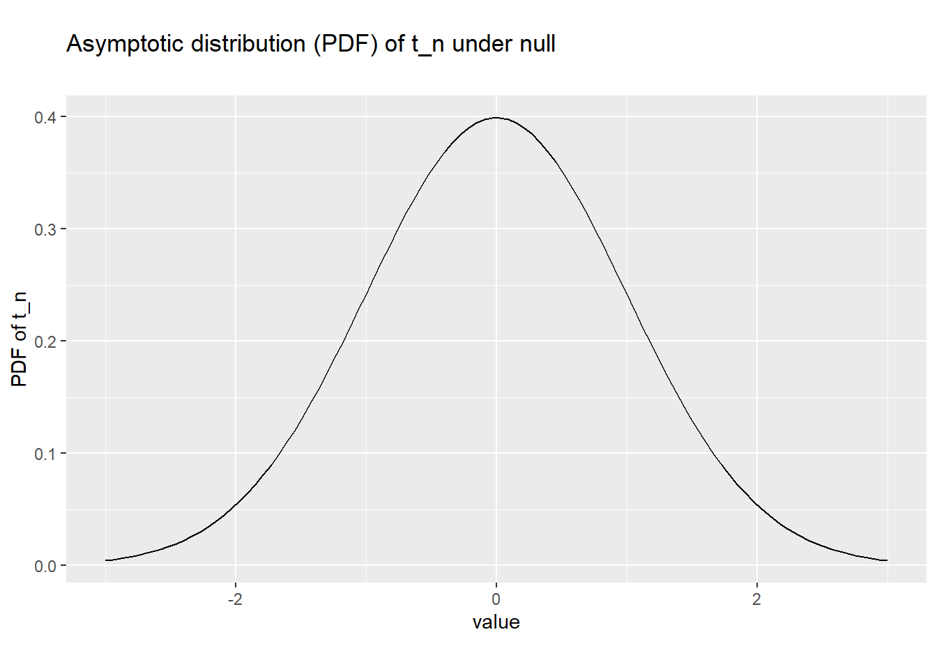
Figure 8.4: Asymptotic distribution of t_n under the null

Therefore, if we want a test that has the asymptotic size of 5%, the critical values should be:

$$\begin{align} c_L &= 2.5 \textrm{ percentile of $N(0,1)$ distribution} \\ c_H &= 97.5 \textrm{ percentile of $N(0,1)$ distribution} \end{align}$$ We can use Excel or R to calculate these critical values. In Excel, the function would be NORM.INV() or NORM.S.INV(), and the formulas would be:

• $c_L$: =NORM.S.INV(0.025) or =NORM.INV(0.025,0,1).
• $c_H$: =NORM.S.INV(0.975) or =NORM.INV(0.975,0,1).

In R, the function would be qnorm() and the code would be:

cat("cL = 2.5 percentile of N(0,1) = ", round(qnorm(0.025), 3), "\n")
## cL = 2.5 percentile of N(0,1) =  -1.96
cat("cH = 97.5 percentile of N(0,1) = ", round(qnorm(0.975), 3), "\n")
## cH = 97.5 percentile of N(0,1) =  1.96

These particular critical values are so commonly used that I want you to remember them.

Example 8.21 The asymptotic test for roulette

We have calculated above that the 5% asymptotic critical values for our roulette test are $c_L = -1.96$ and $c_H = 1.96$. We have also calculated the T statistic for each of our two cases:

Case 1: Red wins 35 of the 100 games, and the test statistic is $t_n \approx -2.84$. This is outside of the critical range $(-1.96,1.96)$, so we reject the null of a fair game.

Case 2: Red wins 40 of the 100 games, and the test statistic is $t_n \approx -1.75$. This is inside of the critical range $(-1.96,1.96)$, so we fail to reject the null of a fair game.

8.4.5 Parametric critical values

Most economic data comes in sufficiently large samples that the asymptotic distribution of $t_n$ is a reasonable approximation and the asymptotic test works well. But occasionally we have samples that are small enough that it doesn’t.

Another option is to assume that the $x_i$ variables are normally distributed: $$\begin{align} x_i \sim N(\mu_x,\sigma_x^2) \end{align}$$ where $\mu_x$ and $\sigma_x^2$ are unknown parameters. Keep in mind that many interesting variables are not normally distributed, so the assumption that $x_i$ is normally distributed is not necessarily appropriate in every setting.

Example 8.22 Normality in the roulette data?

In our roulette data, $x_i$ has the discrete support $\{0,1\}$ and could not possibly be normally distributed. But we will ignore that for the moment.

The null distribution of the test statistic $t_n = \frac{\bar{x}-\mu_0}{s_x/\sqrt{n}}$ under these particular assumptions was derived in the 1920’s by William Sealy Gosset, a statistician working at the Guinness brewery. To avoid getting in trouble at work (Guinness did not want to give away trade secrets) Gosset published under the pseudonym “Student”. As a result, the family of distributions he derived is called “Student’s T distribution”. Gosset’s calculations are beyond the scope of this course. But you should understand the basic idea: the distribution of the T statistic (or any other statistic based on $x_i$) under the null can be derived once we assume a specific distribution for $x_i$.

When the null is true, the test statistic $t_n = \frac{\bar{x}-\mu_0}{s_x/\sqrt{n}}$ has the Student’s T distribution with $n-1$ degrees of freedom: $$\begin{align} (H_0:\mu_x = \mu_0) \qquad \implies \qquad t_n \sim T_{n-1} \end{align}$$ and when the null is false, it has a different distribution which is sometimes called the “noncentral T distribution.”

The $T_{n-1}$ distribution looks a lot like the $N(0,1)$ distribution, but has slightly higher probability of extreme positive or negative values (a statistician would say the distribution has “fatter tails”). As $n$ increases, the extreme values become less common and the $T_{n-1}$ distribution converges to the $N(0,1)$ distribution as predicted by the Central Limit Theorem.

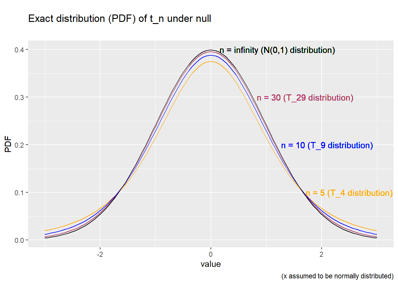
Figure 8.5: Distribution of t_n under the null, parametric test

Having found our test statistic and its distribution under the null, we can calculate our critical values: $$\begin{align} c_L &= 2.5 \textrm{ percentile of the $T_{n-1}$ distribution} \\ c_H &= 97.5 \textrm{ percentile of the $T_{n-1}$ distribution} \end{align}$$ We can obtain these percentiles using Excel or R. The relevant function in Excel is T.INV and the relevant function in R is qt().

Example 8.23 Calculating critical values for the $T$ distribution

If we have $n = 5$ observations, then we can calculate critical values in Excel:

• We would calculate $c_L$ by the formula =T.INV(0.025,5-1).
• We would calculate $c_H$ by the formula =T.INV(0.975,5-1).

or in R:

cat("cL = 2.5 percentile of T_4 = ", round(qt(0.025, df = 4), 3), "\n")
## cL = 2.5 percentile of T_4 =  -2.776
cat("cH = 97.5 percentile of T_4 = ", round(qt(0.975, df = 4), 3), "\n")
## cH = 97.5 percentile of T_4 =  2.776

In contrast, if we have 30 observations, then:

• We would calculate $c_L$ by the formula =T.INV(0.025,30-1).
• We would calculate $c_H$ by the formula =T.INV(0.975,30-1).

The results (calculated below using R) would be:

## cL = 2.5 percentile of T_29 =  -2.045
## cH = 97.5 percentile of T_29 =  2.045

and if we have 1,000 observations:

• We would calculate $c_L$ by the formula =T.INV(0.025,1000-1).
• We would calculate $c_H$ by the formula =T.INV(0.975,1000-1).

The results (calculated below using R) would be:

## cL = 2.5 percentile of T_999 =  -1.962
## cH = 97.5 percentile of T_999 =  1.962

Notice that with 1,000 observations the parametric critical values are nearly identical to the asymptotic critical values. That is, the normality assumption matters less and less as the sample size increases.

Once we have calculated critical values, all that remains is to implement the test.

Example 8.24 A parametric test for roulette

As mentioned earlier, our roulette data are definitely not normally distributed. But suppose we do not realize this, and assume normality anyway. Since we have 100 observations, this normality assumption implies that our test statistic $t_n = \frac{\bar{x}-\mu_0}{s_x/\sqrt{n}}$ has a Student’s T distribution with 99 degrees of freedom: $$\begin{equation} H_0 \qquad \implies \qquad t_n \sim T_{99} \end{equation}$$ We can then calculate critical values for a 5% test:

## cL = 2.5 percentile of T_99 =  -1.984
## cH = 97.5 percentile of T_99 =  1.984

We can then apply these to our two cases:

Case 1: Red wins in 35 of the 100 games, and the test statistic is $t_n \approx -2.84$. This is outside of the critical range $(-1.98,1.98)$, so we reject the null of a fair game.

Case 2: Red wins in 40 of the 100 games, the test statistic is $t_n \approx -1.75$. This is inside of the critical range $(-1.98,1.98)$, so we fail to reject the null of a fair game.

8.4.6 Choosing a test

Statisticians often call the parametric test for the mean the T test and the asymptotic test the Z test, as a result of the notation typically used to represent the test statistic. The two tests have the same underlying test statistic, but different critical values. So which test should we use in practice?

• For any finite value of $n$, the T test is the more conservative test.
  • It has larger critical values than the Z test.
  • It is less likely to reject the null.
  • It has lower power and lower size.
• At some point (around $n \approx 30$) the difference between the two tests becomes too small to make much of a difference.
• In the limit (as $n \rightarrow \infty$) the two tests are equivalent.

As a result, statisticians typically recommend using the T test for smaller samples (less than 30 or so), and then using whichever test is more convenient with larger samples. Most data sets in economics have well over 30 observations¹³, so economists tend to use asymptotic tests unless they have a very small sample.

Example 8.25 Choosing a test for roulette

We have developed three tests for the fairness of a roulette game:

1. An exact test based on the win count and the binomial distribution.
2. A parametric test based on the T statistic and the Student’s T distribution.
3. An asymptotic test based on the T statistic and the standard normal distribution.

In a purely technical sense, the exact test is preferable: it is based on the true distribution of the test statistic under the null, while the other two tests are based on approximations. But it is more difficult to implement.

In the end, all three tests produced the same results: we reject the null of a fair game if red wins 35 times out of 100, and fail to reject that null if red wins 40 times out of 100. This should make sense, as the three tests are just slightly different ways of assessing the same evidence. If all three tests are reasonable ways of assessing the evidence, they should reach the same conclusion in all but a few borderline cases.

8.5 Confidence intervals

Hypothesis tests have one very important limitation: although they allow us to rule out $\theta = \theta_0$ for a single value of $\theta_0$, they say nothing about other values very close to $\theta_0$.

For example, suppose you are a medical researcher trying to measure the effect of a particular cancer treatment. Let $\theta$ be the true effect, and suppose that you have tested the null hypothesis that the treatment has no effect ($\theta = 0$).

• If you reject this null, you have concluded that the effect has some effect.
  • This does not rule out the possibility that the effect is very small.
  • If the treatment is very costly or has harmful side effects, you may not want to use it even if it has a small positive effect.
• If you fail to reject this null, you cannot rule out the possibility that the treatment has no effect.
  • This does not rule out the possibility that the effect is very large.
  • If the treatment is very cheap, or the prognosis without treatment is very poor, you may want to use it even if you cannot be sure it has an effect.

One solution to this would be to do a hypothesis test for every possible value of $\theta$, and classify them into values that were rejected and not rejected. This is the idea of a confidence interval.

A confidence interval for the parameter $\theta$ with coverage rate $CP$ is an interval with lower bound $CI_L$ and upper bound $CI_H$ constructed from the data in such a way that: $$\begin{align} \Pr(CI_L < \theta < CI_H) = CP \end{align}$$ In economics and most other social sciences, the convention is to report confidence intervals with a coverage probability of 95%. $$\begin{align} \Pr(CI_L < \theta < CI_H) = 0.95 \end{align}$$ We might choose to report a 99% confidence interval when we have a lot of data, or a 90% confidence interval when we have very little data.

How do we calculate confidence intervals? It turns out to be entirely straightforward: confidence intervals can be constructed by inverting hypothesis tests:

• The 95% confidence interval includes all values that cannot be rejected at a 5% level of significance.
• The 90% confidence interval includes all values that cannot be rejected at a 10% level of significance.
  • It is narrower than the 95% confidence interval.
• The 99% confidence interval includes all values that cannot be rejected at a 1% level of significance.
  • It is wider than the 95% confidence interval.

Confidence intervals can be constructed using exact tests, asymptotic tests, or parametric tests.

Example 8.26 An exact confidence interval for the win probability

Calculating an exact confidence interval for $p_{red}$ requires a computer. The details are beyond the scope of this course, but the procedure looks like this:

1. Construct a grid of many values between 0 and 1.
2. For each value $p_0$ in the grid, test the null hypothesis $H_0: p_{red} = p_0$ against the alternative hypothesis $H_1: p_{red} \neq p_0$.
3. The confidence interval is the range of values for $p_0$ that are not rejected.

Just to give you an idea how this might be implemented, here is the R code and its results:

# Construct a grid of many values between 0 and 1
theta <- seq(0, 1, length.out = 101)
# For each value in the grid, test the null hypothesis
cL <- qbinom(0.025, 100, theta)
cH <- qbinom(0.975, 100, theta)
accept35 <- (cL < 35 & cH > 35)
accept40 <- (cL < 40 & cH > 40)
# The confidence interval is the range of values that are not rejected
thetaCI35 <- range(theta[accept35])
thetaCI40 <- range(theta[accept40])
# If red wins 35 games:
cat("95% CI for win probability: ", thetaCI35[1], " to ", thetaCI35[2], "\n")
## 95% CI for win probability:  0.27  to  0.44
# If red wins 40 games:
cat("95% CI for win probability: ", thetaCI40[1], " to ", thetaCI40[2], "\n")
## 95% CI for win probability:  0.32  to  0.49

Notice that the confidence interval for 40 wins includes the fair value of 0.486 but it also includes some very unfair values. In other words, while we are unable to rule out the possibility that we have a fair game, the evidence that we have a fair game is not very strong.

8.5.1 Confidence intervals for the mean

Asymptotic confidence intervals for the mean are very easy to calculate. Again, we construct them by inverting the hypothesis test.

Pick any $\mu_0$. We would fail to reject the null hypothesis $H_0: \mu_x = \mu_0$ if our test statistic $t_n = \sqrt{n}\frac{\bar{x}-\mu_0}{sd_x}$ is inside the critical range $[c_L,c_H]$

To summarize, we fail to reject the null if: $$\begin{align} c_L < \sqrt{n}\frac{\bar{x}-\mu_0}{sd_x} < c_H \end{align}$$ The next step is to solve¹⁴ for $\mu_0$: $$\begin{align} \left(\bar{x} - c_H \frac{sd_x}{\sqrt{n}}\right) < \mu_0 < \left(\bar{x} - c_L \frac{sd_x}{\sqrt{n}}\right) \end{align}$$ All that remains is to choose a confidence/size level, decide whether to use a parametric or asymptotic test, and calculate critical values.

If we wish to construct a 95% confidence interval using an asymptotic test, then the 5% asymptotic critical values are $c_L = -1.96$ and $c_H \approx 1.96$. So the 95% asymptotic confidence interval consists of all $\mu_0$ such that: $$\begin{align} \left(\bar{x} - 1.96 \frac{sd_x}{\sqrt{n}}\right) < \mu_0 < \left(\bar{x} - (-1.96) \frac{sd_x}{\sqrt{n}}\right) \end{align}$$ A more compact way of stating this result is: $$\begin{align} CI^{95} = \bar{x} \pm 1.96 \frac{sd_x}{\sqrt{n}} \end{align}$$ In other words, the 95% confidence interval for $\mu_x$ is just the point estimate plus or minus roughly 2 standard errors.

Example 8.27 An asymptotic confidence interval for the win probability

The 5% critical values for the $N(0,1)$ distribution are $c_L \approx -1.96$ and $c_H \approx 1.96$, so the 95% asymptotic confidence intervals for our two cases are:

Case 1: Red wins 35 of 100 games ($\bar{x} = 0.35$ and $s_x \approx 0.479$). The asymptotic confidence interval for the win probability is: $$\begin{align} CI &= \bar{x} \pm 1.96 \frac{s_x}{\sqrt{n}} \\ &\approx 0.35 \pm 1.96 \frac{0.479}{\sqrt{100}} \\ &\approx [0.256, 0.443] \end{align}$$ Case 2: Red wins 40 out of 100 games ($\bar{x} = 0.40$ and $s_x \approx 0.492$). The asymptotic confidence interval for the win probability is: $$\begin{align} CI &= \bar{x} \pm 1.96 \frac{s_x}{\sqrt{n}} \\ &\approx 0.40 \pm 1.96 \frac{0.492}{\sqrt{100}} \\ &\approx [0.304, 0.496] \end{align}$$ These asymptotic confidence intervals are sightly wider than the exact confidence intervals derived earlier in this section.

If we have a small sample, and choose to assume normality rather than using the asymptotic approximation, then we need to use the slightly larger critical values from the $T_{n-1}$ distribution.

Example 8.28 A parametric confidence interval for the win probability

The 5% critical values for the $T_{99}$ distribution are $c_L \approx -1.98$ and $c_H \approx 1.98$, so the 95% parametric confidence intervals for our two cases are:

Case 1: Red wins 35 out of 100 games ($\bar{x} = 0.35$ and $s_x \approx 0.479$), so the parametric 95% confidence interval for the win probability is: $$\begin{align} CI &= \bar{x} \pm 1.98 \frac{s_x}{\sqrt{n}} \\ &\approx 0.35 \pm 1.98 \frac{0.479}{\sqrt{100}} \\ &\approx [0.255, 0.445] \end{align}$$ Case 2: Red wins 40 out of 100 games ($\bar{x} = 0.40$ and $s_x \approx 0.492$), so the parametric 95% confidence interval for the win probability is: $$\begin{align} CI &= \bar{x} \pm 1.98 \frac{s_x}{\sqrt{n}} \\ &\approx 0.40 \pm 1.98 \frac{0.492}{\sqrt{100}} \\ &\approx [0.303, 0.497] \end{align}$$ These parametric confidence intervals are slightly wider than the asymptotic confidence intervals derived earlier in this section.

In the end, it rarely matters much whether you base your confidence intervals on an exact, parametric or asymptotic test. Again this makes sense: the goal here is to assess the strength of the evidence in a given data set, so any two reasonable approaches should yield similar results most of the time.

Chapter review

Hypothesis tests and confidence intervals are important tools for addressing uncertainty in our statistical analysis. In this chapter, we have learned to formulate and test hypotheses, and to construct confidence intervals.

The mechanics are complicated, but do not let the various formulas distract you from the more basic idea of evidence: hypothesis testing is about how strong the evidence is in favor of (or against) a particular true/false statement about the data generating process, and confidence intervals are about finding a range of values for a parameter that are consistent with the observed data. Modern statistical packages automatically calculate and report confidence intervals for most estimates, and report the result of some basic hypothesis tests as well. When you need something more complicated, it is usually just a matter of looking up the command. The most important skill is to correctly interpret the results.

This is the last primarily theoretical chapter in this book, so congratulations for making it this far. The remaining chapters will be data-oriented and will help you build your computer skills.

Practice problems

Answers can be found in the appendix.

GOAL #1: Select a parameter of interest, null hypothesis, and alternative hypothesis

1. Suppose we have a research study of the effect of the minimum wage on employment. Let $\beta$ be the parameter defining that effect. Formally state a null hypothesis corresponding to the idea that the minimum wage has no effect on employment, and state the alternative hypothesis as well.

GOAL #2: Identify the properties of a valid test statistic

2. Which of the following characteristics do test statistics need to possess?
   1. The distribution of the test statistic is known under the null.
   2. The distribution of the test statistic is known under the alternative.
   3. The test statistic has the same distribution whether the null is true or false.
   4. The test statistic has a different distribution when the null is true versus when the null is false.
   5. The test statistic needs to be a number that can be calculated from the data.
   6. The test statistic needs to have a normal distribution.
   7. The test statistic’s value depends on the true value of the parameter.

GOAL #3: Find distribution of a simple test statistic under the null and alternative

3. Suppose we have a random sample of size $n$ on the random variable $x_i$ with unknown mean $\mu$ and unknown variance $\sigma^2$. The conventional T-statistic for the mean is defined as: $$\begin{align} t = \frac{\bar{x}-\mu_0}{sd_x/\sqrt{n}} \end{align}$$ where $\bar{x}$ is the sample average, $\mu_0$ is the value of $\mu$ under the null, and $sd_x$ is the sample standard deviation.
   1. What needs to be true in order for $t$ to have the $T_{n-1}$ distribution under the null?
   2. What is the asymptotic distribution of $t$?
4. Consider the setting from problem 3 above, and suppose that the true value of $\mu$ is some number $\mu_1 \neq \mu_0$. Write an expression describing $t$ as the sum of (a) a random variable that has the $T_{n-1}$ distribution and (b) a random variable that is proportional to $\mu_1-\mu_0$.

GOAL #4: Find the size/significance of a simple test

5. Suppose that we have a random sample of size $n=14$ on the random variable $x_i \sim N(\mu,\sigma^2)$. We wish to test the null hypothesis $H_0: \mu = 0$. Suppose we use the standard t-statistic: $$\begin{align} t = \frac{\bar{x}-\mu_0}{sd_x/\sqrt{n}} \end{align}$$
   1. Suppose we use critical values $c_L = -1.96$ and $c_H = 1.96$. Use Excel to calculate the exact size of this test.
   2. Suppose we use critical values $c_L = -1.96$ and $c_H = 1.96$. Use Excel to calculate the asymptotic size of this test.
   3. Suppose we use critical values $c_L = -3$ and $c_H = 2$. Use Excel to calculate the exact size of this test.
   4. Suppose we use critical values $c_L = -3$ and $c_H = 2$. Use Excel to calculate the asymptotic size of this test.
   5. Suppose we use critical values $c_L = -\infty$ and $c_H = 1.96$. Use Excel to calculate the exact size of this test.
   6. Suppose we use critical values $c_L = -\infty$ and $c_H = 1.96$. Use Excel to calculate the asymptotic size of this test.

GOAL #5: Find critical values for a test of given size

6. Suppose that we have a random sample of size $n=18$ on the random variable $x_i \sim N(\mu,\sigma^2)$. We wish to test the null hypothesis $H_0: \mu = 0$. Suppose we use the standard t-statistic: $$\begin{align} t = \frac{\bar{x}-\mu_0}{sd_x/\sqrt{n}} \end{align}$$
   1. Use Excel to calculate the (two-tailed) critical values that produce an exact size of 1%.
   2. Use Excel to calculate the (two-tailed) critical values that produce an exact size of 5%.
   3. Use Excel to calculate the (two-tailed) critical values that produce an exact size of 10%.
   4. Use Excel to calculate the (two-tailed) critical values that produce an asymptotic size of 1%.
   5. Use Excel to calculate the (two-tailed) critical values that produce an asymptotic size of 5%.
   6. Use Excel to calculate the (two-tailed) critical values that produce an asymptotic size of 10%.

GOAL #6: Implement and interpret a hypothesis test

7. Suppose you estimate the effect of a university degree on earnings at age 30, and you test the null hypothesis that this effect is zero. You conduct a test at the 5% level of significance, and reject the null. Based on this information, classify each of these statements as “probably true”, “possibly true”, or “probably false”:
   1. A university degree has no effect on earnings.
   2. A university degree has some effect on earnings.
   3. A university degree has a large effect on earnings.
8. Suppose you estimate the effect of a university degree on earnings at age 30, and you test the null hypothesis that this effect is zero. You conduct a test at the 5% level of significance, and fail to reject the null. Based on this information, classify each of these statements as “probably true”, “possibly true”, or “probably false”:
   1. A university degree has no effect on earnings.
   2. A university degree has some effect on earnings.
   3. A university degree has a large effect on earnings.

GOAL #7: Construct and interpret a confidence interval

9. Suppose we have a random sample of size $n = 16$ on the random variable $x_i \sim N(\mu,\sigma^2)$, and we calculate the sample average $\bar{x} = 4$ and the sample standard deviation $sd_x = 0.3$.
   1. Use Excel to calculate the 95% (exact) confidence interval for $\mu$.
   2. Use Excel to calculate the 90% (exact) confidence interval for $\mu$.
   3. Use Excel to calculate the 99% (exact) confidence interval for $\mu$.
   4. Use Excel to calculate the 95% asymptotic confidence interval for $\mu$.
   5. Use Excel to calculate the 90% asymptotic confidence interval for $\mu$.
   6. Use Excel to calculate the 99% asymptotic confidence interval for $\mu$.
10. Suppose you estimate the effect of a university degree on earnings at age 30, and your 95% confidence interval for the effect is $(0.10,0.40)$, where an effect of 0.10 means a degree increases earnings by 10% and an effect of 0.40 means that a degree increases earnings by 40%. Based on this information, classify each of these statements as “probably true”, “possibly true”, or “probably false”:
    1. A university degree has no effect on earnings.
    2. A university degree has some effect on earnings.
    3. A university degree has a large effect on earnings, where “large” means at least 10%.
    4. A university degree has a very large effect on earnings, where “very large” means at least 50%.

---

12. You may notice that the curves do not exactly cross the point $(18/37,0.05)$. This is because the binomial distribution is discrete, so it is not possible to achieve a size of exactly 5%.↩︎

13. You will sometimes see old textbooks or internet resources treat 30 as some kind of “magic number” at which statistical analysis somehow moves from invalid to valid, or at which the central limit theorem or law of large numbers applies. But this is not the case, it is only the sample size at which the 5% critical values for the $T$ and $N(0,1)$ distributions are approximately the same. But it is entirely possible that both distributions poorly approximate the true distribution of the test statistic, in which case a sample of size 30 only guarantees they provide equally poor approximations.↩︎

14. If you do not remember the rules for algebra with inequalities, they are just like for equality, but the inequality switches sides whenever both sides are multiplied or divided by a negative number. For example, if $a < b$, then $-a > -b$.↩︎