Chapter 5 Basic data analysis with Excel
Once we have cleaned our data we are ready to start analyzing it. Our analysis can include viewing the data, summarizing it in tables, and visualizing it in charts.
This chapter will demonstrate the use of Excel to construct univariate statistics and charts, i.e., statistics and charts that describe a single variable. Later chapters will describe some multivariate methods that can be used to describe the relationship between two or more variables.
Chapter goals
In this chapter, we will learn how to:
- Use Excel tools for viewing larger data tables, including:
- Sorting
- Filtering
- Freezing panes
- Calculate and interpret univariate summary statistics by hand:
- Sample size (count)
- Sample average
- Sample median
- Sample variance and standard deviation
- Calculate univariate summary statistics in Excel.
- Sample size (count)
- Sample average
- Sample range, percentiles, and median
- Sample variance and standard deviation
- Construct and interpret simple and binned frequency tables in Excel.
- Construct and interpret time series (line) graphs in Excel.
- Construct and interpret bar graphs and histograms in Excel.
To prepare for this chapter, please review the chapter on basic data cleaning with Excel.
5.1 Viewing large data files
The first step in any data analysis is to literally look at the data. It is easy to miss obvious problems or surprising patterns if you just dive right into calculations.
Example 5.1 Historical employment data for Canada
Our analysis in this chapter will use historical employment data for Canada from January 1976 through January 2021.
- Set up a project folder.
- Download the file at https://bookdown.org/bkrauth/IS4E/sampledata/CanEmpHist.xlsx and put it in your raw data subfolder.
- Make a working copy in your project folder.
- I called mine
CanEmpHist-working.xlsx.
- I called mine
- Open your working copy. It will look something like this:
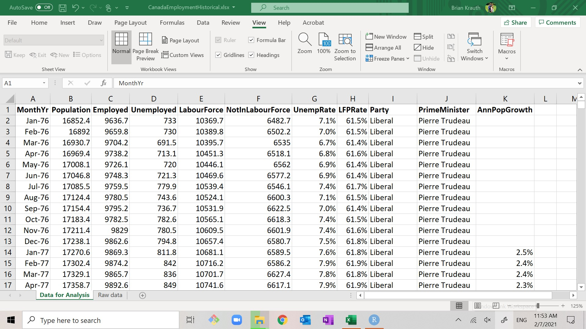
There is a worksheet titled Raw data that contains the original data as obtained from Statistics Canada, along with information on its sources.
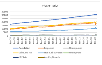
Our main data set for analysis is in the worksheet Data for Analysis, which includes the following variables:
- MonthYr: the month and year of the observation.
- Population: the civilian, non-institutionalized working-age population of Canada at that time, in thousands.
- Employed: the total number employed in the population, in thousands.
- Unemployed: the total number employed in the population, in thousands.
- LabourForce: the sum of Employed and Unemployed.
- NotInLabourForce: the difference between Population and LabourForce.
- UnempRate: the percentage of the labour force that is unemployed. As before, it is calculated and stored as a decimal (ranging from 0.0 to 1.0) but displayed as a percentage (ranging from 0% to 100%).
- LFPRate: the percentage of the population that is in the labour force. As before, it is calculated and stored as a decimal (ranging from 0.0 to 1.0) but displayed as a percentage (ranging from 0% to 100%).
- Party: the political party in control of the Federal government. If the party in control changed during the month, it is listed as “Transfer”.
- PrimeMinister: the name of the Prime Minister. If the prime minister changed during the month, it is listed as “Transfer”.
- AnnPopGrowth: the rate of population growth over the previous 12 months, calculated as a proportion and displayed as a percentage. Note that this variable is blank for the first 12 months of the data set.
This data set covers over 500 months, and is much larger than the single month of data we cleaned earlier.
Most data sets of interest are very large. For example, surveys from Statistics Canada can have hundreds of variables and hundreds of thousands of observations, and companies and governments often work with transactions-level data that includes millions or even billions of observations. Humans are smart, but not smart enough to fully understand a large data set without some kind of simplification or “dimension reduction.” Instead of trying to directly interpret thousands or millions of numbers, we will need to calculate and view a relatively small number of statistics based on the data. A statistic is just a number calculated from data.
But before we calculate statistics for our data set, we can use a few Excel tools - sorting, filtering and freezing - to view selected parts of our data set.
5.1.1 Sorting
Sorting allows us to re-order the rows of our data based on the value in one or more of the columns. Since order does not matter with tidy data, we can sort in whatever way we like without changing the content of our data.
Before sorting data, always make sure that the order of rows does not convey important information.
Example 5.2 Sorting the employment data
The original data are ordered by date. But suppose we wanted it to be ordered by unemployment rate (with the highest rate on top) instead. Here’s all we need to do:
- Select any cell in the UnempRate column.
- Select
Home > Sort and Filter > Sort Largest to Smallest.
As you can see, the data set is now sorted by unemployment rate. We can follow similar steps to put the data set back in date order:
- Select any cell in the MonthYr column.
- Select
Home > Sort and Filter > Sort Oldest to Newest.
Notice that Excel can tell whether a column contains numbers, texts or dates, and will sort accordingly.
You can sort in ascending or descending order, and you can sort on multiple columns by selecting the “Custom sort” option.
5.1.2 Filtering
Filtering allows us to hide some observations so we can look at a particular subset of observations that we are interested in. The hidden observations are still there, so this is a much safer option than deleting observations.
Example 5.3 Filtering the employment data
Suppose we only want to see data from when Paul Martin was the Prime Minister. Here’s what we can do:
- Select
Home > Sort and Filter > Filter. If you look at the column headers in your sheet you will see that they have become drop-down boxes. - Click on the drop-down box for PrimeMinister, then uncheck every box
but the one marked
Paul Martin.
At this point, only the months when Paul Martin was the Prime Minister appear in the table. Don’t worry, the other ones haven’t gone anywhere.
We can undo the filter and remove the drop-down boxes by selecting
Home > Sort and Filter > Filter again.
You can filter on more complex criteria, and you can combine sorting and filtering.
5.1.3 Freezing panes
Freezing panes keeps some rows and/or columns visible regardless of which cell is currently selected. This allows us to work with large tables while keeping the top row (variable names) and/or the first column (observation IDs) visible.
Example 5.4 Freezing panes
Go down to row 50 or so in your worksheet. Notice that you cannot see the variable names in row 1 any more. We can make sure the first row stays visible by doing the following:
- Go back to cell A1.
- Select
View > Freeze Panes > Freeze Top Row.
Now go back down to row 50 or so. You will see that the top row is still displayed and you can see the variable names.
To undo this, select View > Freeze Panes > Unfreeze Panes.
Instead of freezing the first row, you can freeze the first column, or you can freeze any number of rows and columns.
5.2 Summary statistics
Next, we will calculate some commonly-used univariate statistics, which are statistics that describe a single variable in isolation. In Section 5.4 we will construct some commonly-used univariate graphs.
A table of summary statistics reports various univariate statistics for each variable in our data set. For example, our table of summary statistics might look like this:
| Statistic | (variable name 1) | (variable name 2) | (etc.) |
|---|---|---|---|
| Count | (count of valid observations) | ||
| Average | (average) | ||
| StdDev | (standard deviation) | ||
| Min | (minimum value observed) | ||
| 10th percentile | |||
| Median | |||
| 90th percentile | |||
| Max | (maximum value observed) |
You saw many of these words - standard deviation, percentile, median, etc. - in Chapter 4, but I need to be clear on something: even though the names are the same, the concepts are not exactly the same.
We start by introducing some notation. We can think of our data set \(D_n = (x_1, x_2, \ldots, x_n)\) as a table of \(n\) observations (rows), numbered by some sequential index \(i\). The value of our variable of interest in row \(i\) is denoted by \(x_i\); for example \(x_1\) is the value of our variable for the observation in the first row, \(x_{10}\) is the value in the tenth row, etc. We can then define various commonly-used statistics based on \(D_n\):
The count or sample size is the number \(n\) of observations with
valid (numeric) values for the variable. It is calculated in Excel using the
COUNT() function.
The sample average is a measure of central tendency in data, and is
calculated:
\[\begin{align}
\bar{x} = \frac{1}{n} \sum_{i=1}^n x_i
\end{align}\]
or in Excel using the AVERAGE() function.
The sample standard deviation is a measure of variation in the data,
and is calculated:
\[\begin{align}
\hat{sd}_x = \sqrt{\frac{1}{n-1} \sum_{i=1}^n (x_i - \bar{x})^2}
\end{align}\]
or in Excel using the STDEV.S() function.
The sample minimum is the lowest value observed in the data, and the
sample maximum is the highest value observed in the data. They can be
calculated in Excel using the MIN() and MAX() functions.
The sample median is another measure of central tendency, and is (roughly) a number that is above half of the observations and below the other half. Its more precise definition is: \[\begin{align} \hat{m} &= \begin{cases} x_{[(n/2) + (1/2)]} & \textrm{if $n$ is odd} \\ \frac{x_{[n/2]} + x_{[(n/2) + 1]}}{2} & \textrm{if $n$ is even} \\ \end{cases} \end{align}\] where \(x_{[k]}\) is the value of \(x_i\) for the \(k\)th-lowest observation in the data set. This formula looks complicated, but it’s just a way of describing how you were probably taught to calculate medians in grade school. For example:
- The sample median of \(D_3 = (4,1,3)\) is \(\hat{m} = 3\).
- The sample median of \(D_4 = (4,1,3,2)\) is \(\hat{m} = 2.5\).
It can be calculated in Excel using the MEDIAN() function.
The sample 10th percentile is (roughly) a number that is above 10% of
observations in the data, and the sample 90th percentile is a number
that is above 90% of observations. Either can be calculated in Excel using the PERCENTILE.INC()
function. I will not give you a precise definition or ask you to calculate
sample percentiles by hand.
Note that the sample average/median/percentiles/etc. describe the values observed in a set of data, and are calculated from that data set. The mean/median/percentiles we learned about in Chapter 4 describe the probability distribution of a random variable and are calculated from that probability distribution. As you might imagine, these two sets of concepts are distinct but related. We will discuss how they are related in Chapter 7. For now, just keep in mind that they are distinct.
5.2.1 Constructing the table
The first step in constructing a table of summary statistics is to create a new blank worksheet and fill in the structure of the table.
Example 5.5 Table setup
To set up the table:
- Create a new blank worksheet.
- You can do this by clicking on the
 button at the bottom of the
screen.
button at the bottom of the
screen.
- You can do this by clicking on the
- Rename the worksheet Summary Statistics.
- You can do this by double-clicking on the tab for your new worksheet. A dialog box will open for you to enter the new name.
- Fill in the first column (cells A1:A9) as in the table above.
The next step is to fill in the row of variable names. We could type them in, but let’s do something more sophisticated and flexible: use a formula to pull the variable names in from the original data set.
Example 5.6 Getting variable names from the data
To fill in the variable name for column B:
- Go to cell B1.
- Type
=but don’t hit<enter>yet. - Use your mouse to select the tab for the Data for Analysis worksheet, and
then select cell G1 in the Data for Analysis worksheet.
- The formula bar now says
='Data for Analysis'!G1
- The formula bar now says
- Select
<enter>.- You should now be back in cell B1 in the Summary statistics worksheet.
- Cell B1 should display UnempRate (the contents of cell G1 in Data for Analysis).
What have we done here? We have constructed a formula that successfully references a cell in another worksheet. Note that the relative references are even copied over correctly.
Excel has many built-in functions to calculate summary statistics.
Example 5.7 Summary statistics for UnempRate
To fill in the statistics for column B:
- Use the
COUNT()function to report the observation count in cell B2.- We will want to use an absolute reference for the rows, and a relative
reference for the columns, so the formula should be
=COUNT('Data for Analysis'!G$2:G$542).
- We will want to use an absolute reference for the rows, and a relative
reference for the columns, so the formula should be
- Use the
AVERAGE()function to report the average unemployment rate in cell B3. - Use the
STDEV.S()function to report the standard deviation of the unemployment rate in cell B4.- There is another built-in Excel function called
STDEV.P()that uses a slightly different formula for the standard deviation: \[\begin{align} sd_x^p = \sqrt{\frac{1}{n} \sum_{i=1}^n (x_i - \bar{x})^2} \end{align}\] We will discuss the difference between these two statistics later.
- There is another built-in Excel function called
- Use the
MIN()function to report the minimum unemployment rate in cell B5. - Use the
PERCENTILE.INC()function to report the 10th percentile of the unemployment rate in cell B6.- Warning: Despite its name, the
PERCENTILE.INC()function takes a quantile (between 0 and 1) rather than a percentile (between 0 and 100) as its argument.
- Warning: Despite its name, the
- Use the
MEDIAN()function to report the median unemployment rate in cell B7. - Use the
PERCENTILE.INC()function to report the 90th percentile of the unemployment rate in cell B8. - Use the
MAX()function to report the maximum unemployment rate in cell B9.
We now have a table that reports all of the major summary statistics calculated for the unemployment rate.
We would also like to calculate summary statistics for other variables. Fortunately, we have set up our table in a way that makes that easy.
Example 5.8 Summary statistics for other variables
To fill in summary statistics for other variables:
- Copy the contents of cells B1:B9 to cells C1:F9.
Now column C contains summary statistics for the labour force participation rate (LFPRate), and columns D through F contain summary statistics for some of the other variables in our data set.
If we wanted to, we could set up the table to calculate summary statistics for all of the variables. But let’s just stop with these, and move on to making the table look a little nicer.
5.2.2 Cleaning up the table
Our table now has all of the information we need, but it is still kind of ugly. Let’s make it look nice and presentable.
The first problem is that the columns may be too narrow or too wide. If a column is too narrow, some of its values will display as “####”. If it is too wide, it will take up too much room.
Example 5.9 Cell size
There are many different ways to adjust row heights and column widths, but here is the simplest:
- Select the whole sheet by clicking on the
 button in its upper left corner.
 - Select
Home > Format > AutoFit Column Widthfrom the menu.
Not only will this make everything fit, it will automatically adjust the width as necessary when anything changes.
The second problem is that the non-numeric variables report error codes like
#DIV/0! or #NUM! for several statistics, and nonsense values for others.
Example 5.10 Error codes
It is usually better to leave something blank than have it display meaningless, confusing or incorrect information. So let’s just delete those columns:
- Select columns D and E.
- Select
Home > Delete > Delete Sheet Columns.
Finally, we might want to make the display formatting a little nicer.
Example 5.11 Display formatting
To make the display formatting a little nicer:
Put the top row in bold.
Put the first column in italics.
Adjust the number display formats to look nice. Remember that the number display format has no effect on the number itself.
- Leave the counts as they are.
- Display the unemployment rate, LFP rate and population growth rate in percentages, rounded to one decimal place.
We now have a nice table of summary statistics that we could put into a Word or PowerPoint document, and share with an audience:
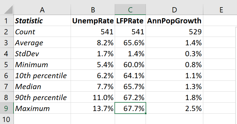 Feel free to play around with colors, fonts, etc. to improve upon this table.
Once you have the table you like, save your working copy.
5.3 Frequency tables
Another way of describing a single variable is a frequency table. A frequency table describes how often different values appear in the data.
5.3.1 Simple frequency tables
A simple frequency table describes how many times each value appears in the data. Simple frequency tables are useful when the underlying variable is discrete, categorical, or even non-numeric, and they look like this:
| (variablename) | Count | Percentage |
|---|---|---|
| (value1) | (# value1) | (% value1) |
| (value2) | (# value2) | (% value2) |
| (value3) | (# value3) | (% value3) |
| etc. |
where:
- The (variablename) column lists all possible values of the variable.
- The Count column reports the number of observations in which the variable matches that value or range of values.
- The Percentage column reports the count as a percentage of the total number of observations.
The Excel functions COUNTIF() and COUNTIFS() can be used to construct the
counts. I will use COUNTIFS() which has a pair of arguments:
- The first argument
criteria_rangegives the range containing the data we want to describe. - The second argument
criteriagives the criteria we want to match.
The kind of criteria you can use are most easily described by examples:
- The formula
=COUNTIFS(A1:A5,"Hello")returns a count of the number of cells in the range A1:A5 that contain the string “Hello”.
- The formula
=COUNTIFS(A1:A5,5)returns a count of the number of cells that contain the number 5. - The formula
=COUNTIFS(A1:A5,">0")returns a count of the number of cells in the range A1:A5 that contain a number greater than zero. - The formula
=COUNTIFS(A1:A5,B1)returns a count of the number of cells in the range A1:A5 that satisfy the criterion given in cell B1.
Example 5.12 A simple frequency table
Let’s create a frequency table for the Party variable in our data set. It should look like this:
| Party | Count | Percentage |
|---|---|---|
| Liberal | (# Liberal) | (% Liberal) |
| Conservative | (# Conservative) | (% Conservative) |
| NDP | (# NDP) | (% NDP) |
| Transfer | (# Transfer) | (% Transfer) |
Note that I have included a political party (the NDP) that is not observed in our data set. We start by setting up the table:
- Create a new sheet named Party control.
- Fill in the top row and first column as in the table above.
Next we will fill in values for the Count column (B):
- Fill in cell B2 using the Excel function
COUNTIFS().- The
criteria_rangewill be the data in our main data set (the Data for Analysis worksheet) covering the Party variable (cell range I2:I542), or'Data for Analysis'!I2:I542. - The
criteriawe want to match is the contents of the cell in the current row of column A, orA2. - So the formula to enter in cell B2 is
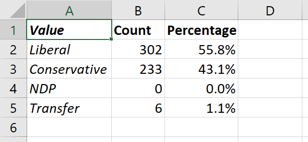
=COUNTIFS('Data for Analysis'!I2:I542,A2). - The result displayed should be 302, the number of observations in our data that have the Party identified as Liberal.
- The
- We will want to copy the formula in cell B2 to the other cells in column B.
But before we do that, we need to make some of the relative references into
absolute references. In this case, our table will keep the same
criteria_rangebut will want to change thecriteria, so:- Change the formula in cell B2 to
=COUNTIFS('Data for Analysis'!I$2:I$542,A2).
- Change the formula in cell B2 to
- Copy cell B2 to cells B3:B4.
- Check the formulas in those cells to make sure they look right.
Next, we need to fill in the Percentage column (C):
- To do that we just need to divide each cell in the Count column by the sum of
all the cells in that column. So the formula in cell C2 should be
=B2/SUM(B2:B5). - Change relative references to absolute references as needed.
- Copy the formula in cell C2 to cells C3:C5.
- By default, the percentages are displayed as proportions. Change the display format to percentage, with one decimal place.
- Make any other formatting changes you like, and save your working copy.
We now have a simple frequency table for the Party variable:
5.3.2 Binned frequency tables
We can also construct frequency tables for continuous variables or discrete variables with many possible values, but doing so is a little more complicated. We cannot just construct a table with a row for each possible value, since there are many possible values.
Instead, we divide the data’s range of possible or observed values into a set of sub-ranges or bins. Then we can calculate and report the number or percentage of observations that fall within each bin. A binned frequency table looks like this:
| From | To | Count | Percentage |
|---|---|---|---|
| (from1) | (to1) | ||
| (from2) | (to2) | ||
| etc. |
In constructing bins, we need to apply some good judgment, and keep in mind a few requirements and considerations:
- We need the bins to cover the full range of the data. In particular:
- The lower bound of the lowest bin should be lower than the lowest value in the data.
- The upper bound of the highest bin should be higher than the highest value in the data.
- Each bin’s upper bound should be the lower bound of the next bin.
- Boundaries should be addressed in a consistent manner, so that each observation falls into exactly one bin.
- We often want the bins to be equally sized.
- But that isn’t always the case. See the unemployment rate table in the example below; if it used equally sized bins, most of the bins would be empty.
- We often want the upper and lower bounds of the bins to be nice round numbers.
- The number of bins is a matter for judgment, and depends on what kind of
patterns we are aiming to find in the data:
- We may miss broad patterns if we have too many bins.
- We may miss potentially interesting details if we have too few bins.
- The solution is to explore multiple options, and see what patterns you can find out.
Again, we will use COUNTIFS() to construct the counts. But we will need to
take advantage of a feature of COUNTIFS() I have not yet mentioned: it takes
multiple criteria_range and criteria arguments, allowing it to make multiple
comparisons (that’s the difference between COUNTIF() and COUNTIFS()).
Example 5.13 A binned frequency table
Let’s create the following table for the unemployment rate variable:
| From | To | Count | Percentage |
|---|---|---|---|
| 0.0% | 5.0% | ||
| 5.0% | 7.5% | ||
| 7.5% | 10.0% | ||
| 10.0% | 15.0% | ||
| 15.0% | 100.0% |
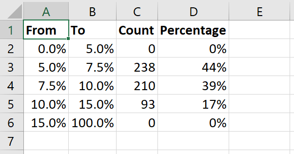
where Count is the number of observations for UnempRate that are greater than that row’s From value and less than or equal to the row’s To value, and Percentage is the count as a percentage of the total. We start by setting up the table:
- Create a new sheet titled Unemployment frequency.
- Copy the first row and first two columns from the table above.
- Enter the From and To values as decimals (0 to 1) and display them as percentages (0% to 100%).
Next, we fill in counts in column C. This will be a somewhat complex formula, so we will build it in stages.
- Let’s start with cell C2. We want this number to contain a count of all observations in which the value of UnempRate is between the value in cell A2 (0%) and the value in cell B2 (5%).
- First, let’s use the
COUNTIFS()function to count the number of observations with UnempRate less than or equal to 5%. TheCOUNTIFS()function takes two arguments:- The
criteria_range1value should be the data range for the UnempRate variable, i.e,'Data for Analysis'!G$2:G$542. Note that I am using absolute references here so that the formula will be copied correctly to other cells. - The
criteria1value should be the string “<=0.05”. - So the formula in cell C2 should be
=COUNTIFS('Data for Analysis'!G$2:G$542, "<=0.05")
- The
- Next, let’s modify the formula in cell C2 so that it only counts the
observations with UnempRate less than or equal to 5% and greater than
or equal to 0%. We can do this by adding a second pair of arguments to
our
COUNTIFS()function. The formula is:
=COUNTIFS('Data for Analysis'!G$2:G$542, "<= 0.05", 'Data for Analysis'!G$2:G$542, ">= 0.00"). If we giveCOUNTIFS()multiple criteria, it will count the number of cases that meet all of the criteria. - Next, let’s modify the formula in cell C2 so that the literal numbers 0.00
and 0.05 are replaced with the contents of cells A2 and B2 respectively.
We can use the
CONCAT()function to concatenate the text “<=” with the number in the relevant cell. For example if cell B2 contains the number 0.05, the formulaCONCAT("<= ",B2)will return the text value<= 0.05. The revised formula in cell C2 should now be:=COUNTIFS('Data for Analysis'!G$2:G$542, CONCAT("<= ",B2), 'Data for Analysis'!G$2:G$542, CONCAT(">= ",A2)). - The formula in cell C2 does what we wanted, so let’s copy it to cell C3.
- The formula in cell C3 is
=COUNTIFS('Data for Analysis'!G$2:G$542, CONCAT("<= ",B3), 'Data for Analysis'!G$2:G$542, CONCAT(">= ",A3)). - Unfortunately, there is a problem. If there are any observations with an unemployment rate exactly equal to 5%, it will be counted in cell C2 and again in cell C3.
- We can fix this issue by modifying the formula in cell C3 to
=COUNTIFS('Data for Analysis'!G$2:G$542, CONCAT("<= ",B3), 'Data for Analysis'!G$2:G$542, CONCAT("> ",A3)). Note that we do not want to modify the formula in cell C2.
- The formula in cell C3 is
- We can finish up by copying the formula in cell C3 to cells C4:C6. You can check your work by confirming that the total of cells C2:C6 adds up to the total number of observations (541).
- Fill in the Percentage column (D) with the appropriate formula and change its display format to Percent.
- Make any other formatting changes you like, and save your working copy.
We now have our binned frequency table:
The FREQUENCY() function is another way to create a frequency table. However,
this function is a tricky one to learn, and Microsoft recently changed how it
works. So we will skip it.
5.4 Univariate graphs in Excel
Another way to explore our data is by visualizing it: constructing and viewing graphs. In this section, we will construct and view three graphs that are useful for understanding a single variable: the time series graph, the bar/column graph, and the histogram. We will also discuss some basic principles for producing presentation-quality graphs.
5.4.1 Charts in Excel
Excel calls graphs charts. Excel charts have three main components:
- The data source. This is the table containing the data used to
construct the graph.
- The individual columns in the data source are called series.
- The chart type. There are many chart types in Excel, but we will use
just a few:
- Line graphs have categories on the horizontal axis, and the value of a variable/series on the vertical axis. Values are depicted by a line connecting the values of the series at each category.
- Column charts have categories on the horizontal axis, and the value of a variable or series on the vertical axis. Values are depicted by a vertical bar for each value of the series.
- Bar charts are just column charts with the axes reversed.
- Scatter or XY charts plot the value of one series against the value of another series. Values can be depicted as a set of points, as a connected line, or both.
- The chart elements, which are the different pieces of the chart.
- Chart elements can be added, removed, or modified.
- The available elements vary across chart types, but can include axes, titles, legends, gridlines, and text labels.
The usual workflow here is to select the data, choose a chart type, and then modify chart elements until the chart looks the way you want it.
5.4.2 Time series (line) graphs
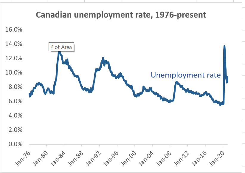
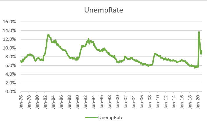
A time series graph plots one or more variables at multiple points in
time. Conventionally, time is on the horizontal axis and the variable’s value
is on the vertical axis. For example, we will generate a time series graph that
looks like this:
In Excel, time series graphs can be implemented using either the Line chart type or the Scatter chart type. Line graphs are simpler, so we will start with that. We will learn how to make scatter plots in Chapter 11.
The first step in creating an Excel chart is to select the data source and graph type.
Example 5.14 Creating a time series graph for UnempRate
We want to create a time series graph for our variable UnempRate.
Select any cell in the Data for analysis table.
Select
Insert > Recommended Chartsfrom the menu.The dialog box will show a few recommended charts. None of them are what we want, so select the
All Chartstab at the top to see the full set of options.Select
Lineto see the line graph options.The dialog box gives you several different types of line graph. Select the picture that looks like this:
and select
OK.
We have our time series graph (it looks like the picture above). Unfortunately, it has a line for every variable in our data source. We only want to plot one variable, so let’s get rid of the others:
- Select
Chart Design > Select Datawhich will open theSelect Data Sourcedialog box. - Uncheck the check box next to every series in the “Legend Entries (Series)”
box except UnempRate, and then select
OK:
This looks like the graph we want.
5.4.3 Creating presentation-quality graphs
The graph we have right now is perfectly fine for exploratory data analysis - using graphs and other tools to better understand the data. However, if we want to convey our understanding to others we need to fine-tune the presentation of our data. Like other elements of a presentation, graphs should be clear, informative, concise, and professional in appearance.
The field of data visualization was pioneered by the statistician Edward Tufte and studies how best to visually convey information. A full discussion of data visualization is beyond the scope of this course, but we can talk about and apply a few basic ideas:
- Clarity: Make all information provided clear to the reader.
- Completeness: Provide all necessary information.
- Simplicity: Remove all repeated, irrelevant or misleading elements (what Tufte calls “chartjunk”).
- Closeness: Minimize eye movement by keeping related information visually “close.”
- Reinforcement: Use color and formatting to reinforce interpretation rather than to complicate it.
- Accessibility: Take reader needs into account. For example:
- Color is not always available to readers: Some readers are color
blind, projectors often get colors “wrong”, or your document
may be printed on a black-and-white printer.
- Always include non-color visual cues (for example, text labels) so that readers who cannot distinguish color (for whatever reason) can tell different series apart.
- Consider using a color palette that is colorblind-friendly.
- A simple way to do this is to avoid using red and green as contrasting colors, since this is the most common form of colorblindness (blue/yellow colorblindness is also common).
- The geographer Cynthia Brewer has developed a set of colorblind-friendly palettes known as ColorBrewer. They are available at https://colorbrewer2.org/.
- Readers in their 50’s and above often have difficulty reading small text.
- Avoid squeezing important text into a tight space.
- Generate graphics that can be re-scaled.
- Readers may have more general and severe visual impairments.
- Provide alt text for all images.
- Color is not always available to readers: Some readers are color
blind, projectors often get colors “wrong”, or your document
may be printed on a black-and-white printer.
Example 5.15 Preparing our graph for presentation
Let’s start by removing unnecessary chart elements.
- Select the chart. This will cause the
Chart DesignandFormatmenu items to appear in the menu. - To remove the horizontal gridlines, select
Chart Design > Add Chart Element > Gridlines > Primary Major Horizontal. - To remove the legend, select
Chart Design > Add Chart Element > Legend > None.
Next, let’s modify the title to be more informative. Right now, it is not clear from the graph what country’s unemployment rate this is.
- Select the title.
- Type in the new title, and hit the
<enter>key.- I went with the title Canadian unemployment, 1976-present
- I also made it boldface.
Next, let’s modify the horizontal axis to be a little less busy:
- Double-click on the horizontal axis. The
Format Axisbox should appear to the right.- It may take you more than one try to double-click on the correct object.
- Select
Axis Options.- You can see all of the choices Excel made here based on what it sees in the data.
- Feel free to play around with these options. You can return each option to
its original/default state by clicking on that option’s
Resetbutton.
- Change the major units to either 4 Years or 8 Years, whichever one you like better.
Finally, let’s add a text label for our time series:
- Select the chart.
- Select
Format > Insert Text Boxfrom the menu. The cursor will change into one that looks like this: - Draw the text box at the desired location on the chart and enter the text “Unemployment rate”
- Resize and move the box to just above the line for the time series.
- Change the color of the text to the same color as the line.
This isn’t really necessary, and violates our principle of avoiding repeated information. But it is useful when we are graphing multiple time series in the same chart, as it is more direct than a legend.
Finally, we want to add alt text for the visually impaired.
- Select the chart.
- Select
Format > Alt Text. The Alt Text dialog box will open to the right. - Enter the alt text in the box.
- I used Graph of Canadian unemployment rate from January 1976 to present.
- Make any other formatting changes you like, and save your working copy.
The graph will now look like the one above. The graph here is visually clean and simple, in part because I left out many elements that I could have included: axis labels (not needed because the units are obvious from context), a fancy background, etc.
One consideration that often comes up when constructing graphs is whether the vertical axis should start at zero when the range of data does not reach zero. In our time series graph of the unemployment rate, Excel included 0% by default even though the variable never went below 5%. I could have changed the vertical axis to start at 5%, but decided not to.
There is no strict rule for whether to include zero, but we can consider the general principle described earlier: our graph should be informative and not misleading. For example, setting the vertical axis to run from 0% to 100% (the theoretical range for the unemployment rate) would be misleading because it would flatten out the line graph and lead the reader to mistakenly conclude that the unemployment rate does not vary much.
For further reading
Data visualization skills are valuable in the academic world and in the business world. If you are interested in developing your skills further, you might consider our course ECON 334: Data Visualization and Economic Analysis.
You might also get a book on data visualization. Cole Nussbaumer Knaflic’s Storytelling with Data is aimed at a business audience and uses Excel. Kieran Healy’s Data Visualization is aimed at a primarily academic audience and uses R. Both of them are practical and easy reads, with many examples.
5.4.4 Frequency (bar/column) graphs
Bar graphs are used to represent the frequency distribution of a categorical variable. Bar graphs use bars of different length to represent the value of some aggregate variable in each category.
Bar graphs are produced from a frequency table, as they are a visual depiction of the information in such a table.
They can be produced in Excel using either the Bar chart type or the Column chart type. The difference between the two is that the bars are horizontal in the Bar chart type and vertical in the Column chart type.
Example 5.16 A bar graph of the Party variable
To construct a bar graph of the Party variable:
- Select any cell in the Party control worksheet.
- Select
Insert > Recommended Chartsfrom the menu. - Select the
All Chartstab to see the full list of options. - Select
Columnand then selectOK.
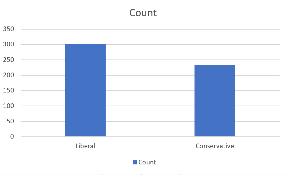
The graph will look something like this:
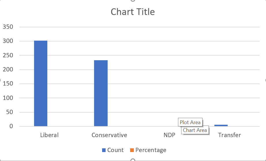
As you can see, basic bar graphs are quite simple. There is a bar for each category (the first column of the table) and variable (the other columns), and the length of each bar corresponds to its value.
As with our line graph, the current graph contains more information than we actually want - it shows the count and the percentage (you can’t see the percentage bars because the percentage is a much smaller number than the count). We really only need one of those. We also may decide that the bars for NDP and “Transfer” ar irrelevant. We can get rid of this irrelevant information:
- Select the chart.
- Select
Chart Design > Select Data. - Uncheck the check boxes for Percentage, NDP and Transfer.
We now have a bar graph that looks like this:
and shows the number of months in which the two largest federal parties were in government over the time frame of our data.
As with line graphs, we can prepare a bar graph for presentation by using Excel’s tools with an eye towards the principles of effective presentation graphics.
Example 5.17 Cleaning up our bar graph
We can do a few easy things to simplify and clarify our bar graph:
- Change the title.
- Remove the gridlines.
- Remove the legend.
- Add the vertical axis title Months in control to clarify the units.
Another thing we can do is use color and branding to convey information: each major Canadian political party has a distinctive color as part of its brand: red for the Liberals, blue for the Conservatives, and orange for the NDP.
- Double-click on the Liberal bar.
- Change its color to red.
- Double-click on the Conservative bar.
- Change its color to blue. The Conservatives use two shades of blue, so pick whichever one you like best.
Finally, the purpose of a bar graph is to enable the viewer to compare magnitudes, which requires looking at the top of each bar. But you may notice that the category labels are at the bottom of each bar. Following the principle that we don’t want to make the reader’s eye do any extra work, let’s put those labels on top.
- Select the chart.
- Select
Chart Design > Add Chart Element > Data Labels > More data label options.
You will notice the numbers 302 and 233 (the heights of the two bars) appear above the bars, and theFormat Data Labelsbox will appear to the right. - Select
Label optionsfrom the dialog box. - Uncheck
Valueand checkCategory Name. The category names Liberal and Conservative will now appear above the respective bar. - Select
Chart Design > Add Chart Element > Axes > Primary Horizontalto eliminate the category names from the bottom of each bar. - You might also consider changing the color of the two labels to match the color of the corresponding bar.
- Make any other formatting changes you like, and save your working copy.
Our final graph looks like this:
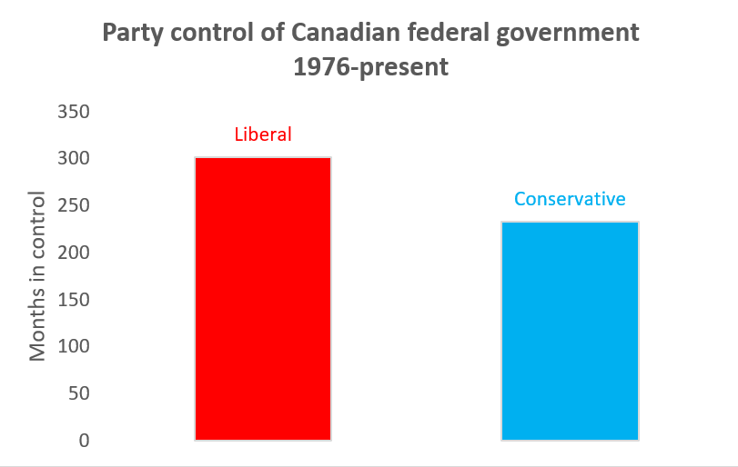
One of the keys to effective bar graph design is to keep the graph simple and clean, and to avoid “chartjunk.”
Bar graphs should always start at zero. The size of the bar is meant to visually represent the value of the variable it is depicting. Using any origin other than zero can cause relative sizes to be misleading.
Example 5.18 Why bar graphs should always start at zero
Suppose we start our Party bar graph at 200 rather than zero. We will get
this:
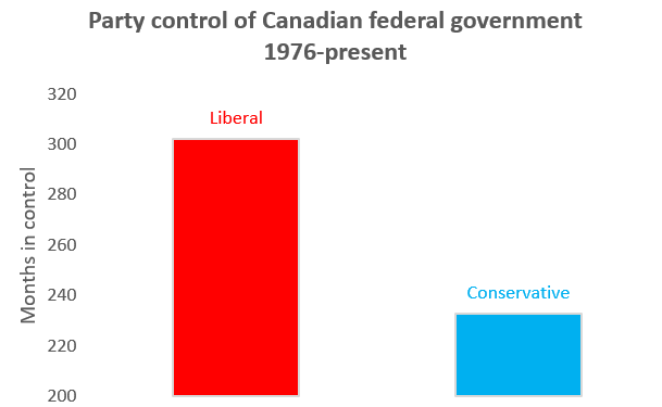
The relative size of these bars is very misleading. The bar for Liberal is three times as big as the bar for Conservative, even though the number it represents is only 29% higher.
Pie graphs are an alternative way of depicting relative frequencies, and are also available in Excel along with 3-dimensional variations on both pie and bar graphs:
| Graph type | Example |
|---|---|
| Pie graph | 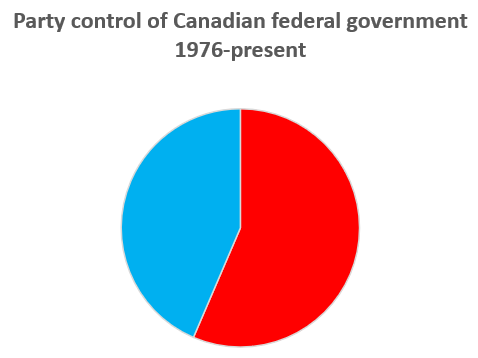 |
| 3D pie graph | 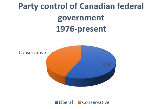 |
| 3D bar graph | 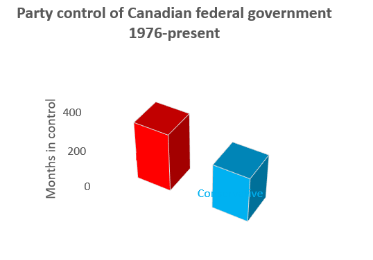 |
However, most data visualization experts recommend against their use. Research on how people process visual information usually find that they are less informative in practice. People are much better at evaluating the relative size of two lines or rectangles than they are at evaluating the relative size of two pie slices. They are also much better at assessing relative distances in two dimensions than they are in three dimensions.
5.4.5 Histograms
A histogram is just a frequency bar/column graph for a continuous variable. It is constructed by sorting the variable’s values into some number of equally-sized bins and then plotting a bar for each bin that represents counts or percentages.
The histogram is a built-in chart type in Excel.
Example 5.19 Constructing a histogram for UnempRate
To construct a histogram of the UnempRate variable:
- Select column G in the Data for Analysis worksheet.
- Notice that for the other charts we could just select any cell in this worksheet. For some reason, this won’t work with the histogram chart type.
- Select `Insert > Recommended Charts” from the menu bar.
- Select the
All Chartstab to see the full set of options. - Select
Histogramand thenOK.
Our graph will appear:
There are two main choices in histogram design:
- How many bins and how should they be determined?
- Should we depict frequencies as counts or percentages?
Excel allows us to customize the bins in various ways. Unfortunately, Excel histograms depict frequencies as counts, and do not easily allow for them to be displayed as percentages. We will use R to generate those histograms.
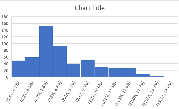
Example 5.20 Changing the bins for a histogram
By default, Excel has chosen 12 equally-sized bins, and each covers 0.73 percentage points. This is a reasonable starting point, but we may find another choice will produce a more informative histogram.
First, let’s try varying the number of bins.
- Select or double-click on the horizontal axis to open the “Format Axis” box.
- Select
Axis Options. - Select
Number of binsand change the number from 12 to something else.- Try a large number like 100 to see what a lot of small bins looks like.
- Try a small number like 5 to see what a few large bins look like.
Looking at these graphs, a relatively large number of bins is needed to accurately convey the distribution of the unemployment rate. But using a lot of bins makes the horizontal axis very busy and difficult to read. One alternative that will help is to fix the bin size at some nice round number like 1% (0.01) or 0.5% (0.005).
- Select or double-click on the horizontal axis to open the
Format Axisbox. - Select
Axis Options. - Select
Bin widthand change the number to 0.01.
Now the bins are exactly one percentage point wide, which makes the horizontal axis a little easier to read and interpret.
It would also be nice to modify the start and end points so that instead of the bins being 5.4-6.4%, 6.4-7.4%, etc. they were 5-6%, 6-7%, etc. Unfortunately, that does not seem to be possible in Excel. We can work around that limitation by creating a binned frequency table, and making a column/bar chart of that table.
Finally, as with other graphs we will want to add, delete and modify various elements to bring this histogram closer to presentation quality.
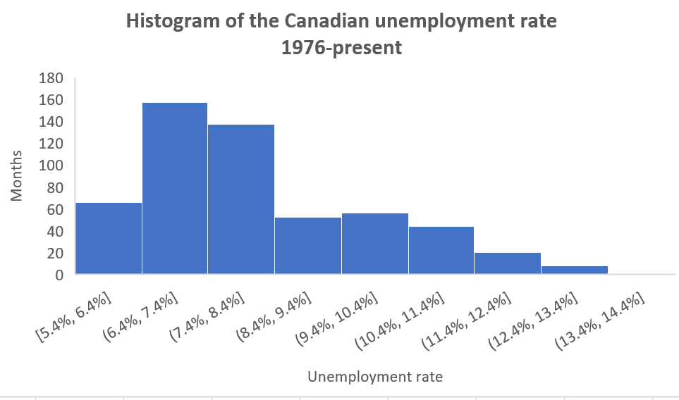
Example 5.21 Enhancing the quality of our histogram
To enhance the quality of this histogram:
- Add/modify the title to Histogram of the Canadian unemployment rate, 1976-present.
- Add the horizontal axis title Unemployment rate.
- Add the vertical axis title # of months.
- Make any other formatting changes you like, and save your working copy.
Our final histogram will look like this:
5.5 Finishing up
As we do when cleaning data, the final steps of a data analysis are to:
- Check your work.
- Update your master version.
Example 5.22 Finishing up our employment data analysis
- Select
Files > Save Asto save your file as the master version. Choose a new name for the file.- I chose the file name
CanEmpHistResults.xlsx.
- I chose the file name
You can download https://bookdown.org/bkrauth/IS4E/sampledata/CanEmpHistResults.xlsx if you want to check your work against mine.
Chapter review
Statistical analysis does not need to be complex to be useful. Simple univariate statistics and graphs can tell us a great deal about the economy.
In this chapter, we learned how to calculate simple statistics in Excel, and how to construct simple graphs. Calculating the statistics is typically the easiest part of a statistical analysis - cleaning data and interpreting the results is much more challenging.
Later in the course, we will bring theory and data together by interpreting the statistics calculated in this chapter as random variables. We will also move beyond the univariate statistics and graphs described in this chapter by developing tools for multivariate data analysis in both Excel and R.
Practice problems
Answers can be found in the appendix.
GOAL #1: Use Excel tools for viewing larger data tables
- Open a copy of the historical unemployment data file CanEmpHist.xlsx. Use sort and filter to show only those months with unemployment rates over 12.5%, sorted in descending order by unemployment rate (i.e., highest unemployment rates at the top).
GOAL #2: Calculate and interpret univariate summary statistics by hand
Consider the following table of data:
Name Age Al 25 Betty 32 Carl 78 Use a calculator or pencil and paper to calculate the following statistics:
- Sample size.
- Sample average age.
- Sample median of age.
- Sample variance of age.
- Sample standard deviation of age.
GOAL #3: Calculate univariate summary statistics in Excel
Consider the following table of data:
Name Age Al 25 Betty 32 Carl 78 Enter this table in Excel, and use Excel functions to to calculate the following statistics:
- Sample size.
- Sample average age.
- Sample median of age.
- Sample 25th percentile of age.
- Sample variance of age.
- Sample standard deviation of age.
GOAL #4: Construct and interpret simple and binned frequency tables in Excel
Consider the following table of data:
Name Age Al 25 Betty 32 Carl 78 Use Excel to construct a binned frequency table of age, with bin widths of 10 years.
GOAL #5: Construct and interpret time series (line) graphs in Excel
Consider the following table of data:
Year Al’s age 2017 25 2018 26 2019 27 2020 28 2021 29 Use Excel to construct a time series graph of Al’s age.
GOAL #6: Construct and interpret bar graphs and histograms in Excel
Consider the following table of data:
Name Age Al 25 Betty 32 Carl 78 Use Excel to construct a histogram of age, with bin widths of 10 years.