Chapter 6 More on random variables
In our first few chapters, we developed the fundamental tools for understanding statistics: the practical skills of cleaning data and calculating statistics, and the basic theoretical concepts for thinking about random events and random variables. Over the next few chapters, we will connect these tools by conceptualizing data sets and the statistics calculated as random variables. This connection is what makes statistics a tool for science and not just a set of calculation procedures. The first step in building that connection is to extend our theory of random variables from a single discrete random variable to a wider range of possibilities.
This chapter extends our theory to both continuous random variables and to pairs or groups of random variables.
Chapter goals
In this chapter, we will learn how to:
- Interpret the CDF and PDF of a continuous random variable.
- Know and use the key properties of the uniform distribution.
- Derive the distribution for a linear function of a uniform random variable.
- Know and use the key properties of the normal distribution.
- Derive the distribution for a linear function of a normal random variable.
- Calculate the joint PDF of two discrete random variables from the probability distribution of a random outcome.
- Calculate a marginal PDF from a (discrete) joint PDF.
- Calculate a conditional PDF from a (discrete) joint PDF.
- Interpret joint, marginal, and conditional distributions.
- Determine whether two random variables are independent.
- Calculate the covariance of two discrete random variables from their joint PDF.
- Calculate the covariance of two random variables using the expected value formula.
- Calculate the correlation of two random variables from their covariance.
- Calculate the covariance and correlation of two independent random variables.
- Calculate the expected value of a linear function of two or more random variables.
- Interpret covariances and correlations.
To prepare for this chapter, please review the introductory chapter on random variables.
6.1 Continuous random variables
Many random variables of interest have a continuous support. That is, they can take on any value in a particular range. Examples of such variables include:
- Physical quantities such as distance, mass, volume, or temperature.
- Time values such as the current time or the time it takes to drive to school from your home.
Because continuous random variables can take on any value in a particular range, the chance that they take on any specific value is very low (in fact, it is zero). This makes the math for continuous random variables a little harder, which is why we started with discrete random variables.
Example 6.1 Labour force participation
The labour force participation rate is defined as: \[\begin{align} (\textrm{LFP rate}) = \frac{(\textrm{labour force})}{(\textrm{population})} \times 100\% \end{align}\] It can be any number between 0% and 100%: \[\begin{align} S_{LFP rate} = [0\%,100\%] \end{align}\] so it is a continuous random variable.
6.1.1 General properties
We can describe the general properties of a continuous random variable by comparing them to the properties of a discrete random variable.
We learned in an earlier chapter that the support of a discrete random variable typically includes a finite number of values, each of which has strictly positive probability, and most formulas for probabilities (including PDFs and CDFs) and expected values use just addition and subtraction.
In contrast, the support of a continuous random variable includes an infinite number of values, each of which has zero probability, and most formulas for probabilities and expected values use calculus.
ECON 233 calculus prerequisites
Differential calculus (MATH 151 or 157) is a prerequisite for ECON 233, but integral calculus (MATH 152 or 158) is not. I will not assume you know how to interpret or calculate an integral, and will not require you to do so in any assigned or graded work in ECON 233.
But deep down, there is no important practical difference between continuous and discrete random variables. The intuition for this is that you can closely approximate any continuous random variable by rounding it. The rounded variable will be discrete, and our earlier results for discrete random variables apply. With only a few exceptions, everything that is true for discrete random variables is also true for continuous ones.
Example 6.2 Rounding a continuous variable to make it discrete
Suppose you round the labour force participation rate to the nearest percentage point. The rounded LFP rate is a discrete random variable with support: \[\begin{align} S_{roundedLFP} = \{0\%, 1\%, \ldots 99\%, 100\% \} \end{align}\] Alternatively, we could round to the nearest 1/100th of a percentage point, to the nearest 1/1,000,000th of a percentage point, etc. As we round to a higher and higher precision, the approximation gets closer and closer.
As a result, our coverage of continuous random variables will be brief and will mostly avoid calculus.
Formulas using integrals
When a relevant mathematical formula uses integrals, I will put it in an “FYI” box like this one. This means I am providing the formula to show you that it exists, but do not expect you to understand, remember, or perform any calculation using the formula.
If you do know some integral calculus, you might notice that the formulas for continuous random variables look just like the ones for discrete random variables, but with sums replaced by integrals. This should not be surprising since an integral is a sum, or at least the limit of a sequence of sums.
6.1.2 The continuous CDF
The CDF of a continuous random variable \(x\) is defined exactly the same way as for the discrete case: \[\begin{align} F_x(a) = \Pr(x \leq a) \end{align}\] The only difference is how it looks. If you recall, the CDF of a discrete random variable takes on a stair-step form: increasing in discrete jumps at every point in the discrete support, and flat everywhere else. In contrast, the CDF of a continuous random variable increases smoothly over its support. It can have flat parts, but it never jumps.
Example 6.3 The standard uniform distribution
Consider a random variable \(x\) that has continuous support: \[\begin{align} S_x = [0, 1] \end{align}\] and CDF: \[\begin{align} F_x(a) = \Pr(x \leq a) = \begin{cases} 0 & a < 0 \\ a & a \in [0,1] \\1 & a > 1 \\ \end{cases} \end{align}\] This particular probability distribution is called the standard uniform distribution and will be discussed in more detail later.
Figure 6.1 shows the CDF of the standard uniform distribution. As you can see, this CDF is smoothly increasing over the support between zero and one, and is flat everywhere else.
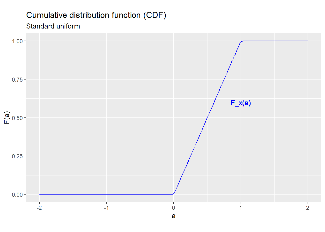
Figure 6.1: CDF for the standard uniform distribution
Section 4.2.2 describes the properties of a CDF, and these properties apply to continuous random variables too. In addition, interval probabilities are easier to calculate for continuous random variables: the probability of any specific value is zero, so it does not matter whether inequalities are strict (\(<\)) or weak (\(\leq\)).
Example 6.4 Interval probabilities for the standard uniform
Suppose that \(x\) has the standard uniform distribution. What is the probability that \(x\) is strictly between 0.65 and 0.70?
We can use our usual formula for interval probabilities to get: \[\begin{align*} \Pr(0.65 < x < 0.70) &= \underbrace{\Pr(0.65 < x \leq 0.70)}_{=F_x(0.70)-F_x(0.65)} - \underbrace{\Pr(x = 0.70)}_{=0} \\ &= 0.70 - 0.65 + 0 \\ &= 0.05 \end{align*}\] So a standard uniform random variable has a 5% chance of being between 0.65 and 0.70.
6.1.3 The continuous PDF
While the CDF has the same definition whether the random variable is discrete or continuous, the same does not hold for the PDF.
- In the discrete case, the PDF \(f_x(a)\) is defined as the size of the “jump” in the CDF at \(a\), or (equivalently) the probability \(\Pr(x=a)\) of observing that particular value.
- In the continuous case, there are no jumps, and the probability of observing any specific value is always zero. So a PDF based on \(\Pr(x=a)\) would be useless in describing the probability distribution of a continuous random variable.
Instead, the PDF of a continuous random variable \(x\) is defined as as the slope or derivative of the CDF: \[\begin{align} f_x(a) = \frac{d F_x(a)}{da} \end{align}\] In other words, instead of the amount the CDF increases (jumps) at \(a\), it is the rate at which it (smoothly) increases.
Example 6.5 The PDF of the standard uniform distribution
The PDF of a standard uniform random variable is: \[\begin{align} f_x(a) = \begin{cases} 0 & a < 0 \\ 1 & a \in [0,1] \\ 0 & a > 1 \\ \end{cases} \end{align}\] Figure 6.2 shows the PDF of the standard uniform distribution.
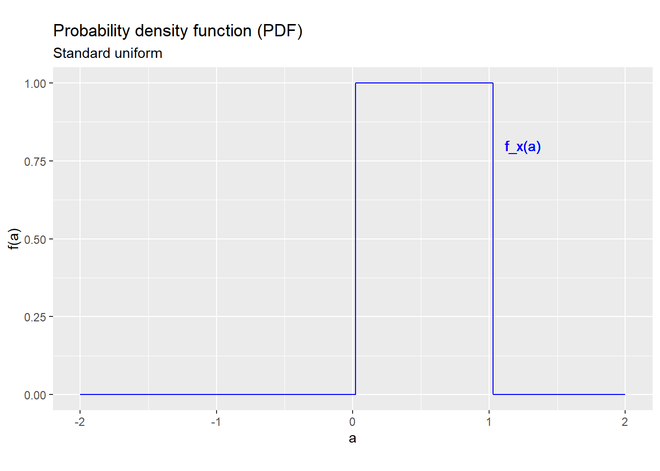
Figure 6.2: PDF for the standard uniform distribution
The PDF of a continuous random variable is a good way to visualize its probability distribution, and this is about the only way we will use the continuous PDF in this class (since everything else requires integration).
Example 6.6 Interpreting the standard uniform PDF
The standard uniform PDF shows the key feature of this distribution: in some loose sense, all values in the support are “equally likely”, much like in the discrete uniform distribution described earlier. In fact, if you round a uniform random variable, you get a discrete uniform random variable.
Like the discrete PDF, the continuous PDF is always non-negative: \[\begin{equation*} f_x(a) \geq 0 \qquad \textrm{for all $a \in \mathbb{R}$} \end{equation*}\] and is strictly positive on the support: \[\begin{equation*} f_x(a) > 0 \qquad \textrm{for all $a \in S_x$} \end{equation*}\] But unlike the discrete PDF, the continuous PDF is not a probability. In particular, it can be greater than one.
Additional properties of the continuous PDF
If you recall, we can calculate probabilities from the discrete PDF by addition. We can use this property to derive the CDF and show that the discrete PDF sums to one.
Similarly, we can calculate probabilities from the continuous PDF by integrating: \[\begin{align} \Pr(a < x < b) = \int_a^b f_x(v)dv \end{align}\] which implies that the CDF can be derived from the PDF: \[\begin{align} F_x(a) = \int_{-\infty}^a f_x(v)dv \end{align}\] and that the PDF integrates to one: \[\begin{align} \int_{-\infty}^{\infty} f_x(v)dv = 1 \end{align}\] Unless you have taken a course in integral calculus, you may have no idea what these formulas mean or how to solve them. That’s OK! All you need to know is that they can be solved.
6.1.4 Quantiles
The quantiles of a random variable have the same definition, interpretation, and properties whether the random variable is continuous or discrete. The same applies to percentiles and the median since they are also quantiles. Quantiles are usually easier to calculate for continuous random variables.
Example 6.7 Quantiles for the standard uniform
Suppose that \(x\) has the standard uniform distribution. The \(q\) quantile of \(x\) is: \[\begin{align} F_x^{-1}(q) &= \min \{a \in S_x : F_x(a) \geq q\} \\ &= \min \{a \in [0,1] : a \geq q\} \\ &= \min [q,1] \\ &= q \end{align}\] For example, the median of \(x\) is 0.5, the 10th percentile is 0.10, the 75th percentile is 0.75, etc.
6.1.5 Expected values
The expected value also has the same interpretation and properties whether the random variable is continuous or discrete. The definition is slightly different, and includes an integral.
The expected value for a continuous random variable
When \(x\) is continuous, its expected value is defined as: \[\begin{align} E(x) = \int_{-\infty}^{\infty} af_x(a)da \end{align}\] Notice that this looks just like the definition for the discrete case, but with the sum replaced by an integral sign.
The variance and standard deviation are both defined in terms of expected values, so they also have the same interpretation and properties whether the random variable is continuous or discrete.
6.2 The uniform distribution
The uniform distribution is a continuous probability distribution that is usually written: \[\begin{align} x \sim U(L,H) \end{align}\] where \(L\) and \(H\) are numbers such that \(L < H\). It is also sometimes written \(x \sim Uniform(L,H)\).
The \(U(0,1)\) distribution is also known as the standard uniform distribution.
6.2.1 The uniform PDF
The uniform distribution has continuous support: \[\begin{align} S_x = [L,H] \end{align}\] and continuous PDF: \[\begin{align} f_x(a) = \begin{cases}\frac{1}{H-L} & a \in S_x \\ 0 & \textrm{otherwise} \\ \end{cases} \end{align}\] The uniform distribution can be interpreted as placing equal probability on all values between \(L\) and \(H\).
Example 6.8 The PDF of the \(U(2,5)\) distribution
Suppose that \(x \sim U(2,5)\). Then its support is the range of all values from 2 to 5, and its PDF is: \[\begin{align} f_x(a) = \begin{cases} \frac{1}{3} & 2 < a < 5 \\ 0 & \textrm{otherwise} \\ \end{cases} \end{align}\] which is depicted in Figure 6.3 below.
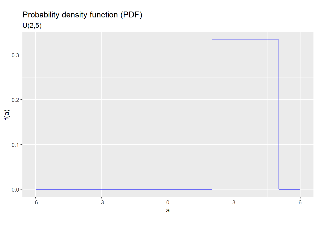
Figure 6.3: PDF for the U(2,5) distribution
6.2.2 The uniform CDF
The CDF of the \(U(L,H)\) distribution is: \[\begin{align} F_x(a) = \begin{cases} 0 & a \leq L \\ \frac{a-L}{H-L} & L < a < H \\ 1 & a \geq H \\ \end{cases} \end{align}\]
Example 6.9 The CDF of the \(U(2,5)\) distribution
The CDF of the \(U(2,5)\) distribution is: \[\begin{align} F_x(a) = \begin{cases} 0 & a \leq 2 \\ \frac{a-2}{3} & 2 < a < 5 \\ 1 & a \geq 5 \\ \end{cases} \end{align}\] and is depicted in Figure 6.4.
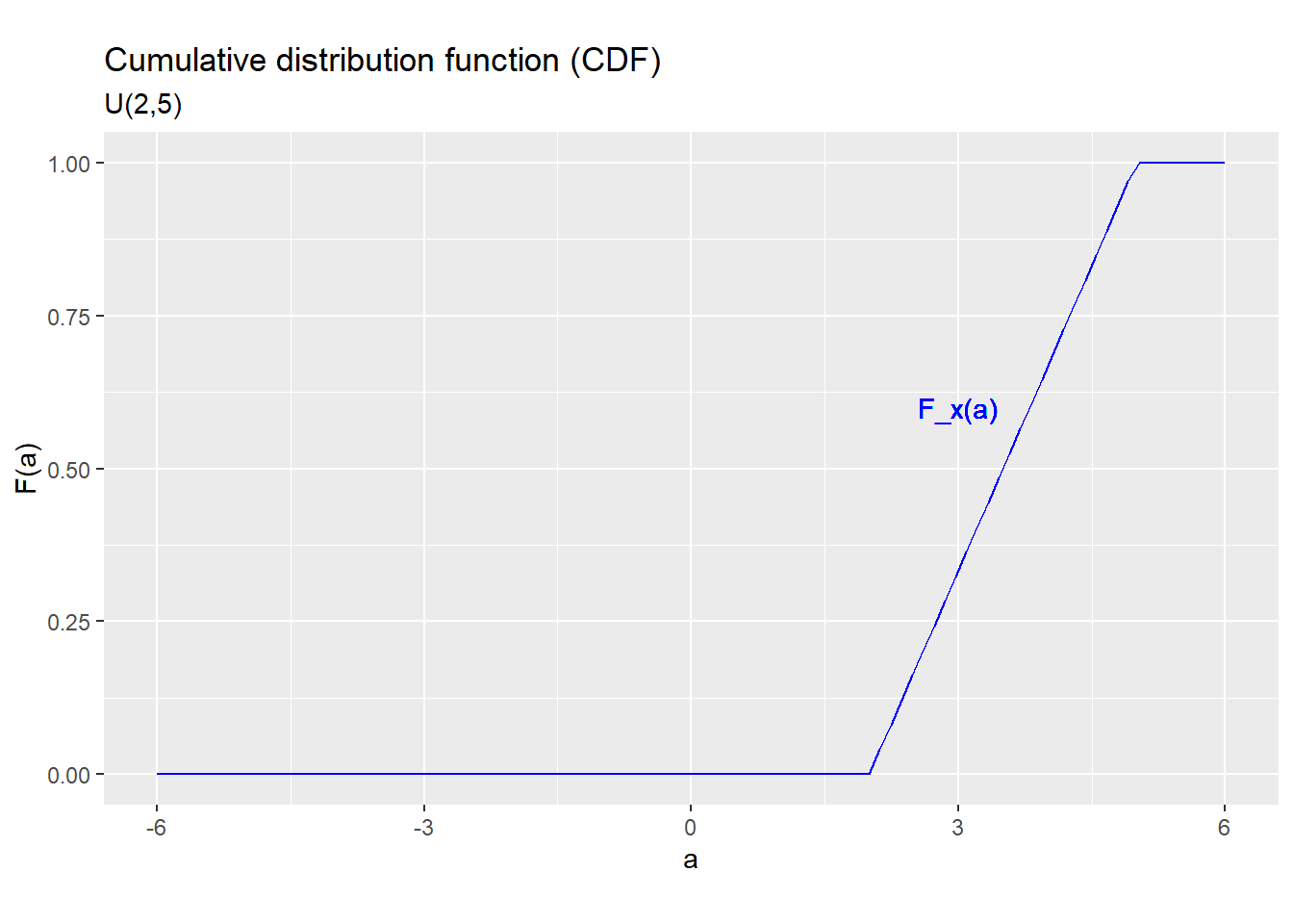
Figure 6.4: CDF for the U(2,5) distribution
6.2.3 Quantiles
Like any other random variable, we can calculate the quantiles of a uniform random variable by inverting the CDF. That is: \[\begin{align} F_x^{-1}(q) = L + q(H-L) \end{align}\] is the \(q\) quantile of a \(U(L,H)\) random variable.
The median of \(x \sim U(L,H)\) is: \[\begin{align} Med(x) = F_x^{-1}(0.5) = 0.5(L+H) \end{align}\] i.e., the midpoint of the support.
Example 6.10 Quantiles of the \(U(2,5)\) distribution
The quantile function of the \(U(2,5)\) distribution is: \[\begin{align} F^{-1}_x(q) = 2 + 3q \end{align}\] and the median is \(F^{-1}_x(0.5) = 3.5\).
6.2.4 Expected values
Integral calculus is required to calculate the mean, variance and standard deviation of the uniform distribution, so I report them below for reference: \[\begin{align*} E(x) &= 0.5(L+H) \\ var(x) &= \frac{(H-L)^2}{12} \\ sd(x) &= \sqrt{\frac{(H-L)^2}{12}} \end{align*}\] This is one advantage of using standard distributions: you can look up results when they are difficult to calculate.
Example 6.11 Expected values of the \(U(2,5)\) distribution
The mean, variance, and standard deviation of the \(U(2,5)\) distribution is: \[\begin{align} E(x) &= 0.5*(2+5) = 3.5 \\ var(x) &= \frac{(5-2)^2}{12} = 0.75 \\ sd(x) &= \sqrt{0.75} = 0.866 \end{align}\]
6.2.5 Functions of a uniform
Any linear function of a uniform random variable also has a uniform distribution. That is, if \(x \sim U(L,H)\) and \(y = a + bx\) where5 \(b > 0\), then: \[\begin{align} y \sim U(a + bL, a + bH) \end{align}\] Nonlinear functions of a uniform random variable are generally not uniform.
Example 6.12 Linear functions of a \(U(2,5)\) random variable
Suppose that \(x \sim U(2,5)\). Then: \[\begin{align} 2x &\sim U(4,10) \\ x + 1 &\sim U(3,6) \\ 2x + 2 &\sim U(6,12) \end{align}\]
Uniform distributions in video games
Uniform distributions are important in many computer applications including video games. Games need to be at least somewhat unpredictable in order to stay interesting.
It is easy for a computer to generate a random number from the \(U(0,1)\) distribution, and that distribution has the unusual feature that its \(q\) quantile is equal to \(q\).
As a result, you can generate a random variable with any probability distribution you like by following these steps:
- Let \(F_{w}(\cdot)\) be the CDF of the distribution you want.
- Generate a random variable \(q \sim U(0,1)\).
- Calculate \(x = F_{w}^{-1}(q)\), where \(F_{w}^{-1}(\cdot)\) is the inverse of \(F_{w}(\cdot)\).
Then \(x\) is a random variable with the CDF \(F_w(\cdot)\)
Any modern video game is constantly generating and transforming \(U(0,1)\) random numbers to determine the behavior of non-player characters, the location of weapons and other resources, or the results of a particular player action.
6.3 The normal distribution
The normal distribution is typically written as: \[\begin{align} x \sim N(\mu,\sigma^2) \end{align}\] where \(\mu\) and \(\sigma^2 \geq 0\) are numbers. It is also sometimes written as \(x \sim Normal(\mu, \sigma^2)\).
The normal distribution is also called the Gaussian distribution, and the \(N(0,1)\) distribution is called the standard normal distribution.
The central limit theorem
An important result called the central limit theorem implies that many “real world” random variables tend to be normally distributed. We will discuss the central limit theorem in much more detail later.
6.3.1 The normal PDF
The \(N(\mu,\sigma^2)\) distribution is a continuous distribution with support
\(S_x = \mathbb{R}\) and PDF:
\[\begin{align}
f_x(a) = \frac{1}{\sigma \sqrt{2\pi}} e^{-\frac{(a-\mu)^2}{2\sigma}}
\end{align}\]
The Excel function NORM.DIST() can be used to calculate this PDF.
Figure 6.5 below shows the PDF of the \(N(\mu,\sigma^2)\) distribution for various values of \(\mu\) and \(\sigma\). As the figure shows, the Normal PDF is bell-shaped and symmetric around \(\mu\), with the “spread” of the distribution depending on the value of \(\sigma^2\).
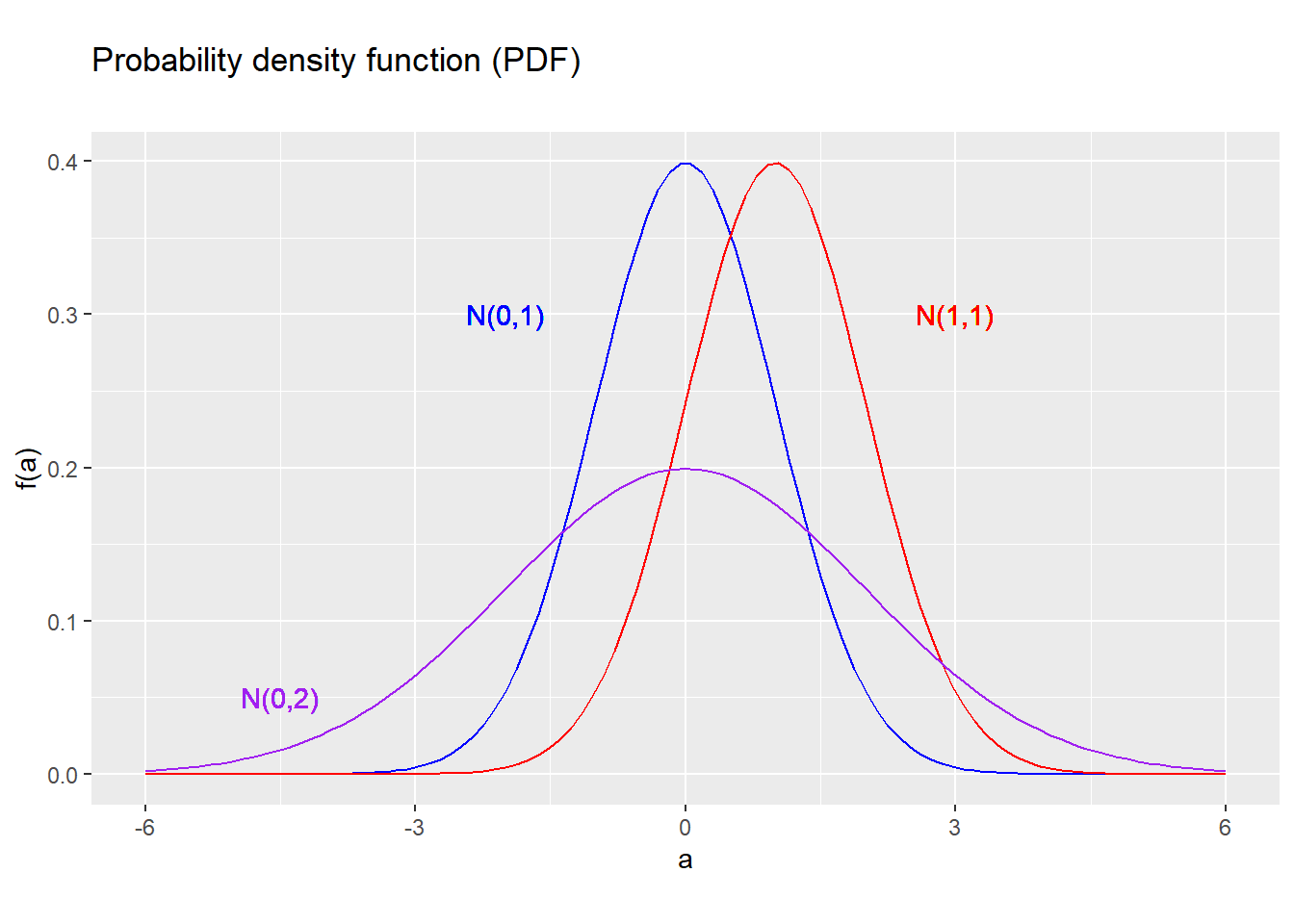
Figure 6.5: PDF for several normal distributions
6.3.2 The normal CDF
The CDF of the normal distribution can be derived by integrating the PDF. There
is no simple closed-form expression for this CDF, but it is easy to calculate
with a computer. The Excel function NORM.DIST() can be used to calculate this
CDF.
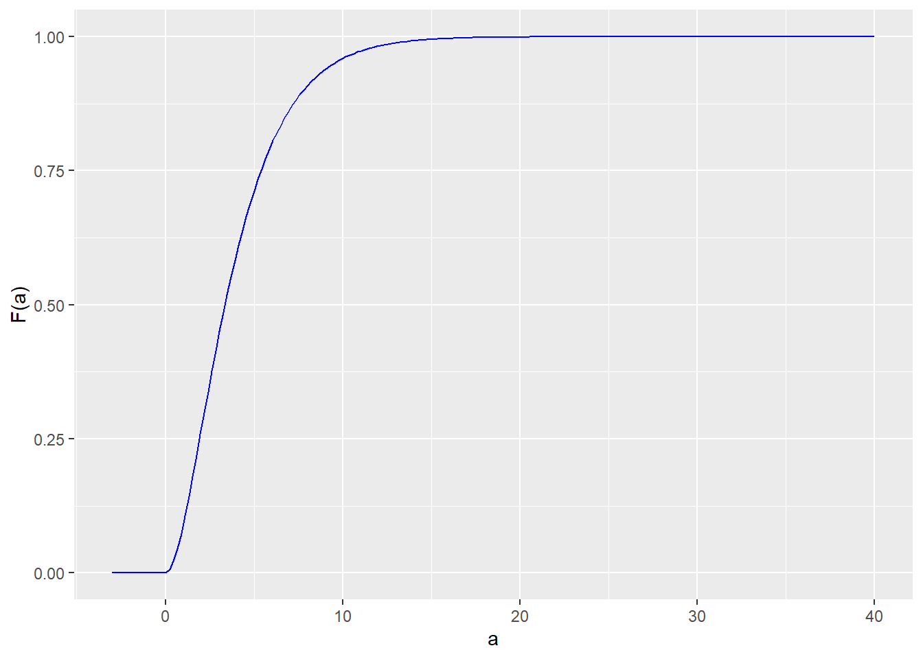
Figure 6.6 below shows the CDF of the \(N(\mu,\sigma^2)\) distribution for various values of \(\mu\) and \(\sigma\). As the figure shows, the Normal CDF is S-shaped, running smoothly from nearly-zero to nearly-one.
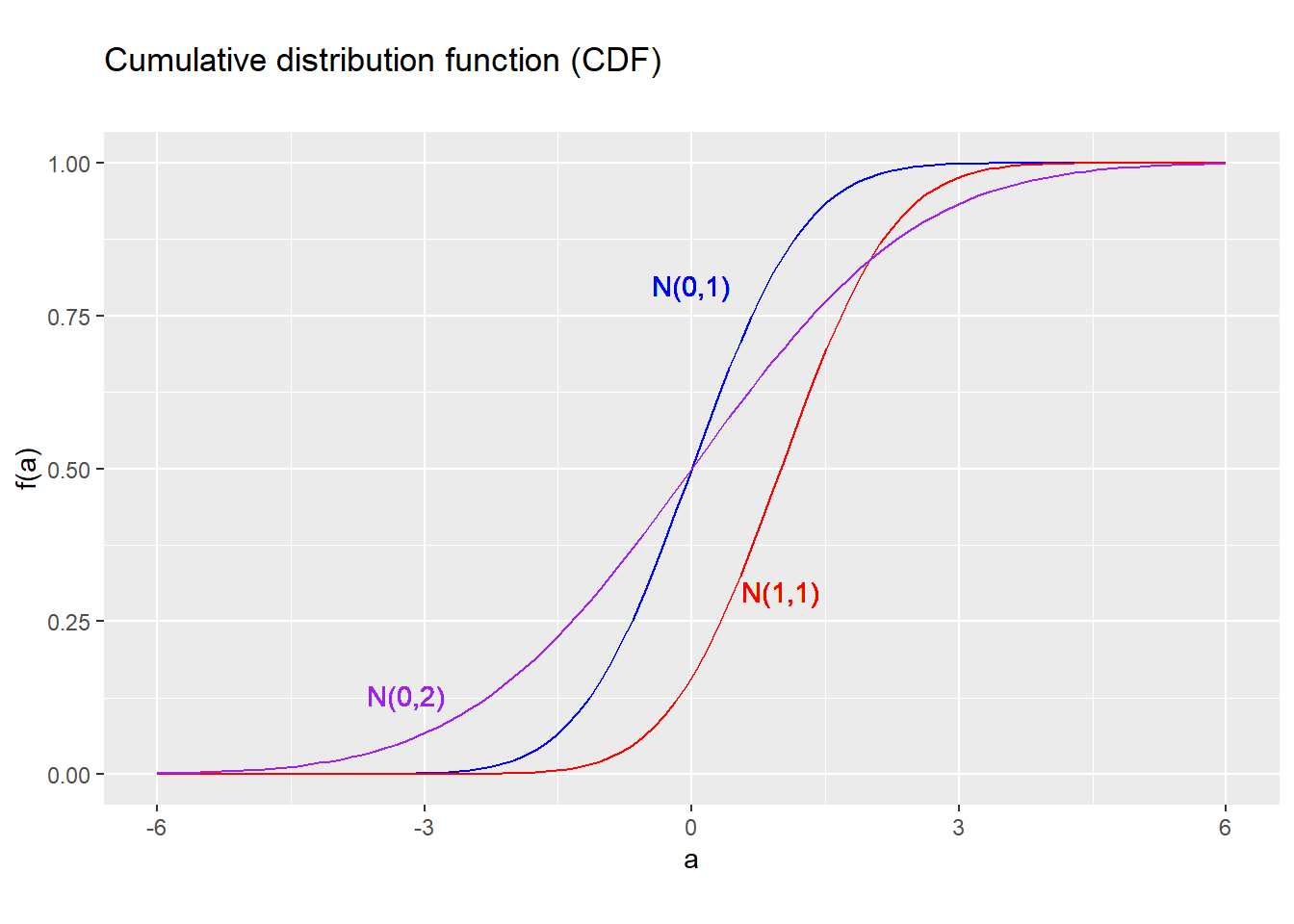
Figure 6.6: CDF for several normal distributions
Example 6.13 The CDF of a normal random variable
Suppose \(x \sim N(2,9)\), and we would like to calculate \(\Pr(x \leq 1)\). We
can use the Excel formula =NORM.DIST(1,2,3,TRUE) to get:
\[\begin{align}
\Pr(x \leq 1) &\approx 0.37
\end{align}\]
6.3.3 Quantiles
Quantiles of the normal distribution can be calculated using the Excel function
NORM.INV().
The median of a \(N(\mu,\sigma^2)\) random variable is \(\mu\).
Example 6.14 Quantiles of a normal random variable
Suppose \(x \sim N(2,9)\). The median of \(x\) is \(\mu = 2\), and its 25th
percentile is:
\[\begin{align}
F^{-1}(0.25) &\approx -0.023
\end{align}\]
which we can calculate using the Excel formula =NORM.INV(0.25,2,3).
6.3.4 Expected values
Integral calculus is required to calculate the mean, variance and standard deviation of the normal distribution, so I report them below for reference: \[\begin{align} E(x) &= \mu \\ var(x) &= \sigma^2 \\ sd(x) &= \sigma \end{align}\]
Example 6.15 Expected values of a normal random variable
Suppose \(x \sim N(2,9)\). Then: \[\begin{align} E(x) &= \mu = 2 \\ var(x) &= \sigma^2 = 9 \\ sd(x) &= \sigma = 3 \end{align}\]
6.3.5 Functions of a normal
As discussed in an earlier chapter, all random variables have the property that \(E(a +bx) = a + bE(x)\) and \(var(a+bx) = b^2 var(x)\) for any constants \(a\) and \(b\).
Normal random variables have an additional property: any linear function of a normal random variable is also normal. That is, if: \[\begin{align} x \sim N(\mu,\sigma^2) \end{align}\] Then for any constants \(a\) and \(b\): \[\begin{align} a + bx \sim N(a + b\mu, b^2\sigma^2) \end{align}\] Nonlinear functions of a normal random variable are generally not normal.
Example 6.16 Linear functions of a normal random variable
Suppose \(x \sim N(2,9)\). Then: \[\begin{align} x + 1 &\sim N(3, 9) \\ 2x &\sim N(4, 36) \\ -2x &\sim N(-4, 36) \end{align}\]
Other distributions based on the normal
There are many other standard distributions that are based on functions of one or more normal random variables and are derived from the normal distribution. For example, if you draw \(k\) independent \(N(0,1)\) random variables, square them, and add them up, the distribution of that sum has a distribution called the \(\chi^2(k)\) distribution.
Other such distributions include the \(F\) distribution and the \(T\) distribution. All of these standard distributions have important applications in statistical analysis and would be covered in a more advanced course.
6.3.6 Standardized normals
We earlier defined the standardized version of a random variable \(x\) as the following linear function of \(x\): \[\begin{align} z = \frac{x-E(x)}{sd(x)} \end{align}\] and showed that \(E(z) = 0\) and \(var(z) = sd(z) = 1\).
We can standardize any random variable, but standardization is particularly convenient for normal random variables. If \(x\) has a normal distribution, then its standardized value \(z\) has the standard normal distribution: \[\begin{align} x \sim N(\mu, \sigma^2) &\Rightarrow z \sim N\left(\frac{\mu-\mu}{\sigma}, \left(\frac{1}{\sigma}\right)^2 \sigma^2\right) \\ &\Rightarrow z \sim N(0,1) \end{align}\] The standard normal distribution is so useful that we have special symbol for its PDF: \[\begin{align} \phi(a) = \frac{1}{\sqrt{2\pi}} e^{-\frac{a^2}{2}} \end{align}\] and its CDF: \[\begin{align} \Phi(a) = \int_{-\infty}^a \phi(b)db \end{align}\] \(\phi\) is the lower-case Greek letter phi, and \(\Phi\) is the upper-case Phi.
We can take advantage of standardization to express the CDF of any normal random variable in terms of the standard normal CDF. That is, suppose that: \[\begin{align} x \sim N(\mu, \sigma^2) \end{align}\] Then we can prove that its CDF is: \[\begin{align} F_x(a) &= \Phi\left(\frac{a-\mu}{\sigma}\right) \end{align}\] The standard normal CDF is available as a built-in function in every statistical package including Excel and R, so we can use this result to calculate the CDF for any normally distributed random variable.
Example 6.17 Obtaining normal probabilities
Suppose \(x \sim N(2,9)\), and we want to find \(F_x(1) = \Pr(x \leq 1)\).
Excel has two built-in functions for the normal distribution:
NORM.DIST()calculates the PDF or CDF for any normal random distribution.NORM.S.DIST()calculates the PDF or CDF for the standard normal distribution.
The easiest way to calculate our probability is with NORM.DIST(), using the
formula =NORM.DIST(1,2,3,TRUE), which yields \(F_x(1) \approx 0.37\).
We can also calculate our probability using only the standard normal CDF
(NORM.S.DIST()) by following these steps:
- Write down the formula, substituting in the correct variable names. \[\begin{align} F_x(1) &= \Phi\left(\frac{1-\mu}{\sigma}\right) \end{align}\]
- Find parameter values and substitute. In this case \(\mu=2\) and \(\sigma^2=9\), so: \[\begin{align} F_x(1) &= \Phi\left(\frac{1-2}{3}\right) \\ &= \Phi\left(-0.333\right) \end{align}\]
- Use the standard normal CDF in Excel or R to calculate the value. In this
case, the formula in Excel would be
=NORM.S.DIST(-0.333,TRUE)which produces: \[\begin{align} F_x(1) &\approx 0.37 \end{align}\]
You may wonder why we bother with these steps when we could have just used
NORM.DIST() to get the same (correct) answer. The short answer is that working
with the standard normal distribution is a skill that is useful later.
The normal and standard normal CDF
The result that any normal random variable \(x \sim N(\mu,\sigma^2)\) has CDF \(\Phi\left(\frac{a-\mu}{\sigma}\right)\) can be proved as follows.
First, define: \[\begin{align} z = \frac{x - \mu}{\sigma} \end{align}\] Since \(z\) is a linear function of \(x\), it is also normally distributed: \[\begin{align} z \sim N\left(\frac{\mu-\mu}{\sigma}, \left(\frac{1}{\sigma}\right)^2 \sigma^2\right) \end{align}\] or equivalently: \[\begin{align} z \sim N(0,1) \end{align}\] Then the CDF of \(x\) is: \[\begin{align} F_x(a) &= \Pr\left(x \leq a\right) \\ &= \Pr\left( \frac{x-\mu}{\sigma} \leq \frac{a-\mu}{\sigma}\right)\\ &= \Pr\left( z \leq \frac{a-\mu}{\sigma}\right) \\ &= \Phi\left(\frac{a-\mu}{\sigma}\right) \end{align}\]
6.4 Multiple random variables
Almost all interesting data sets have multiple observations and multiple variables. So before we start talking about data, we need to develop some tools and terminology for thinking about multiple random variables.
To keep things simple, most of the definitions and examples will be stated in terms of two discrete random variables. The extension to more than two random variables is conceptually straightforward but will be skipped.
6.4.1 Joint distribution
Let \(x\) and \(y\) be two random variables defined in terms of the same underlying random outcome. Their joint probability distribution assigns a value to all joint probabilities of the form: \[\begin{align} \Pr(x \in A \cap y \in B) \end{align}\] for any sets \(A, B \subset \mathbb{R}\).
The joint distribution is the key to talking about \(x\), \(y\) and how they are related. Every concept introduced in this section - marginal distributions, conditional distributions, expected values, covariance, correlation, and independence - can be defined in terms of the joint distribution.
Example 6.18 Four joint distributions
The scatter plots in Figure 6.7 below depict simulation results for a pair of random variables \((x,y)\), with a different joint distribution in each graph.
As you can see, the relationship between the two variables differs in each of these cases: graph A shows two seemingly unrelated variables, graph B shows two variables with a negative relationship, graph C shows two variables with a strong positive relationship, and graph D shows two variables with a strong but nonlinear relationship. We will learn some terminology to describe these four relationships.
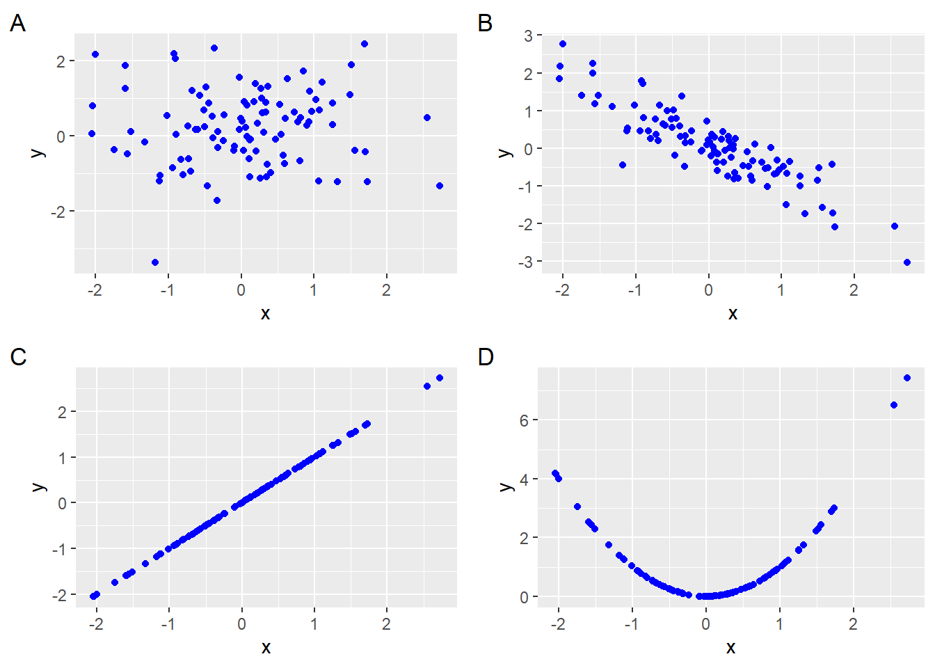
Figure 6.7: x and y are drawn from a different joint distribution in each graph.
The joint distribution of any two discrete random random variables can be fully described by their joint PDF: \[\begin{align} f_{x,y}(a,b) = \Pr(x = a \cap y = b) \end{align}\] The joint PDF can be calculated from the probability distribution of the underlying outcome.
Example 6.19 The joint PDF in roulette
We can derive any joint PDF from the probability distribution of the underlying outcome. In our roulette example, both \(y_{Red}\) and \(y_{14}\) depend on the original outcome \(\omega\), so we can find the joint PDF by following these steps:
- Create a table of outcomes that includes each outcome in the sample space, its probability, and the associated value of our random variables:
| \(\omega\) | \(\Pr(\omega)\) | Color | \(y_{Red}\) | \(y_{14}\) |
|---|---|---|---|---|
| 0 | 1/37 | Green | -1 | -1 |
| 1 | 1/37 | Red | 1 | -1 |
| 2 | 1/37 | Black | -1 | -1 |
| 3 | 1/37 | Red | 1 | -1 |
| 4 | 1/37 | Black | -1 | -1 |
| 5 | 1/37 | Red | 1 | -1 |
| 6 | 1/37 | Black | -1 | -1 |
| 7 | 1/37 | Red | 1 | -1 |
| 8 | 1/37 | Black | -1 | -1 |
| 9 | 1/37 | Red | 1 | -1 |
| 10 | 1/37 | Black | -1 | -1 |
| 11 | 1/37 | Black | -1 | -1 |
| 12 | 1/37 | Red | 1 | -1 |
| 13 | 1/37 | Black | -1 | -1 |
| 14 | 1/37 | Red | 1 | 35 |
| 15 | 1/37 | Black | -1 | -1 |
| 16 | 1/37 | Red | 1 | -1 |
| 17 | 1/37 | Black | -1 | -1 |
| 18 | 1/37 | Red | 1 | -1 |
| 19 | 1/37 | Red | 1 | -1 |
| 20 | 1/37 | Black | -1 | -1 |
| 21 | 1/37 | Red | 1 | -1 |
| 22 | 1/37 | Black | -1 | -1 |
| 23 | 1/37 | Red | 1 | -1 |
| 24 | 1/37 | Black | -1 | -1 |
| 25 | 1/37 | Red | 1 | -1 |
| 26 | 1/37 | Black | -1 | -1 |
| 27 | 1/37 | Red | 1 | -1 |
| 28 | 1/37 | Black | -1 | -1 |
| 29 | 1/37 | Black | -1 | -1 |
| 30 | 1/37 | Red | 1 | -1 |
| 31 | 1/37 | Black | -1 | -1 |
| 32 | 1/37 | Red | 1 | -1 |
| 33 | 1/37 | Black | -1 | -1 |
| 34 | 1/37 | Red | 1 | -1 |
| 35 | 1/37 | Black | -1 | -1 |
| 36 | 1/37 | Red | 1 | -1 |
Add up over outcomes to find the joint PDF.
- There is one outcome (\(b=14\)) in which both red and 14 win, and it has probability \(1/37\): \[\begin{align} f_{Red,14}(1,35) &= \Pr(y_{Red}=1 \cap y_{14} = 35) \\ &= \Pr(\omega \in \{14\}) = 1/37 \end{align}\]
- There are 17 outcomes (count them in the table above) in which red wins and 14 loses, and each has probability \(1/37\): \[\begin{align} f_{Red,14}(1,-1) &= \Pr(y_{Red} = 1 \cap y_{14} = -1) \\ &= \Pr\left(\omega \in \left\{ \begin{gathered} 1,3,5,7,9,12,16,18,19,21,\\ 23,25,27,30,32,34,36 \end{gathered}\right\}\right) \\ &= 17/37 \end{align}\]
- There are 19 outcomes in which both red and 14 lose, and each has probability \(1/37\): \[\begin{align} f_{Red,14}(-1,-1) &= \Pr(y_{Red} = -1 \cap y_{14} = -1) \\ &= \Pr\left(\omega \in \left\{ \begin{gathered} 0,2,4,6,7,10,11,13,15,17, \\ 20,22,24,26,28,31,33,35 \end{gathered}\right\}\right) \\ &= 19/37 \end{align}\]
- There are no other outcomes, so all other combinations have probability zero.
- Summarize results using case notation:
\[\begin{align} f_{Red,14}(a,b) &= \begin{cases} 19/37 & \textrm{if $a = -1$ and $b = -1$} \\ 17/37 & \textrm{if $a = 1$ and $b = -1$} \\ 1/37 & \textrm{if $a = 1$ and $b = 35$} \\ 0 & \textrm{otherwise} \\ \end{cases} \nonumber \end{align}\]
Creating and using the table here is something of a “brute force” approach: it is time consuming, but requires little thought and will always get the right answer. You may be able to figure out a quicker approach, which is also fine.
Other ways of describing a joint distribution
The joint distribution of any two (discrete or continuous) random variables can be fully described by their joint CDF: \[\begin{align} F_{x,y}(a,b) = \Pr(x \leq a \cap y \leq b) \end{align}\]
Similarly, the joint distribution of any two continuous random variables can be fully described by their (continuous) joint PDF: \[\begin{align} f_{x,y}(a,b) = \frac{\partial F_{x,y}(a,b)}{\partial a \partial b} \end{align}\]
6.4.2 Marginal distributions
When two random variables have a joint distribution, we call the probability distribution of each individual random variable its marginal distribution. Both marginal distributions can be derived from the joint distribution: \[\begin{align} \Pr(x \in A) &= \Pr(x \in A \cap y \in \mathbb{R}) \\ \Pr(y \in A) &= \Pr(x \in \mathbb{R} \cap y \in A) \end{align}\] Note that there is no difference between a random variable’s “marginal distribution” and its “distribution”. We just add the word “marginal” in this context to distinguish it from the joint distribution.
The marginal distribution is fully described by the corresponding marginal PDF, which can be derived from the joint PDF. Let \(x\) and \(y\) be two discrete random variables with joint PDF \(f_{x,y}\). Then their marginal PDFs are: \[\begin{align} f_x(a) &= \sum_{b \in S_y} f_{x,y}(a,b) \nonumber \\ f_y(b) &= \sum_{a \in S_x} f_{x,y}(a,b) \nonumber \end{align}\] Pay close attention to where the \(a\) and \(b\) are located when you use these formulas.
Example 6.20 Deriving marginal PDF from joint PDF
We earlier found the joint PDF of \(y_{Red}\) and \(y_{14}\): \[\begin{align} f_{red,14}(a,b) &= \begin{cases} 19/37 & \textrm{if $a = b = -1$} \\ 17/37 & \textrm{if $a = 1$ and $b = -1$} \\ 1/37 & \textrm{if $a = 1$ and $b = 35$} \\ 0 & \textrm{otherwise} \\ \end{cases} \nonumber \end{align}\] Then we can find the marginal PDF of \(y_{Red}\) by following these steps:
- Write down the formula, substituting correct variable names: \[\begin{align} f_{red}(a) &= \sum_{b \in S_b} f_{red,14}(a,b) \end{align}\]
- Find the support and substitute: \[\begin{align} f_{red}(a) &= \sum_{b \in \{-1,35\}} f_{red,14}(a,b) \end{align}\]
- Expand out the summation: \[\begin{align} f_{red}(a) &= f_{red,14}(a,-1) + f_{red,14}(a,35) \end{align}\]
- Find the joint PDF values and substitute: \[\begin{align} f_{red}(-1) &= \underbrace{f_{red,14}(-1,-1)}_{19/37} + \underbrace{f_{red,14}(-1,35)}_{0} \\ &= 19/37 \\ f_{red}(1) &= \underbrace{f_{red,14}(1,-1)}_{17/37} + \underbrace{f_{red,14}(1,35)}_{1/37} \\ &= 18/37 \end{align}\]
- Summarize results using case notation: \[\begin{align} f_{red}(a) &= \begin{cases} 19/37 & \textrm{if $a = -1$} \\ 18/37 & \textrm{if $a = 1$} \\ 0 & \textrm{otherwise} \\ \end{cases} \end{align}\] Note that this is the same PDF we found in an earlier chapter.
While you can always derive the two marginal distributions from the joint distribution, you cannot derive the joint distribution from the two marginal distributions. A given pair of marginal distributions is typically consistent with an infinite number of joint distributions.
Example 6.21 Joint distributions with identical marginal distributions
Graphs A, B and C in Figure 6.7 all depict random variables with the same marginal distribution (both \(x\) and \(y\) have the \(N(0,1)\) distribution in all three graphs) but very different joint distributions.
The joint distribution describes both the individual variables and their relationship.
Example 6.22 Two joint distributions with identical marginal distributions
Suppose Al, Betty, and Carl each place a bet on the same roulette game. Al and Betty both bet on red, and Carl bets on black. Let \(y_{Al}\), \(y_{Betty}\), and \(y_{Carl}\) be their respective winnings.
All three players have the same marginal distribution of winnings: \[\begin{align} f_{Al}(a) = f_{Betty}(a) = f_{Carl}(a) &= \begin{cases} 19/37 & \textrm{if $a = -1$} \\ 18/37 & \textrm{if $a = 1$} \\ 0 & \textrm{otherwise} \\ \end{cases} \end{align}\] since both red and black have a 18/37 chance of winning.
But the joint distribution of \(y_{Al}\) and \(y_{Betty}\): \[\begin{align} f_{Al,Betty}(a,b) &= \begin{cases} 19/37 & \textrm{if $a = -1$ and $b = -1$} \\ 18/37 & \textrm{if $a = 1$ and $b = 1$} \\ 0 & \textrm{otherwise} \\ \end{cases} \end{align}\] is very different from the joint distribution of \(y_{Al}\) and \(y_{Carl}\): \[\begin{align} f_{Al,Carl}(a,b) &= \begin{cases} 1/37 & \textrm{if $a = -1$ and $b = -1$} \\ 18/37 & \textrm{if $a = -1$ and $b = 1$} \\ 18/37 & \textrm{if $a = -1$ and $b = 1$} \\ 0 & \textrm{otherwise} \\ \end{cases} \end{align}\] For example, Betty always wins when Al wins, but Carl always loses when Al wins.
We will soon develop several useful ways of describing the relationship between two random variables including conditional distribution, covariance, correlation, and independence.
Other ways of deriving a marginal distribution
The marginal CDFs of any two random (discrete or continuous) random variables can be derived from their joint CDF: \[\begin{align} F_x(a) &= \lim_{b \rightarrow \infty} F_{x,y}(a,b) \\ F_y(b) &= \lim_{a \rightarrow \infty} F_{x,y}(a,b) \end{align}\] and the marginal PDFs of any two continuous random variables can be derived from their joint PDF: \[\begin{align} f_x(a) &= \int_{-\infty}^{\infty} f_{x,y}(a,b) db \\ f_y(b) &= \int_{-\infty}^{\infty} f_{x,y}(a,b) da \end{align}\]
6.4.3 Conditional distribution
The conditional distribution of a random variable \(y\) given another random variable \(x\) assigns values to all conditional probabilities of the form: \[\begin{align} \Pr(y \in A| x \in B) = \frac{\Pr(y \in A \cap x \in B)}{\Pr(x \in B)} \end{align}\] Since a conditional probability is just the ratio of the joint probability to the marginal probability, the conditional distribution can always be derived from the joint distribution.
The conditional distributions of any two discrete random variables \(x\) and \(y\) can be fully described by the conditional PDF: \[\begin{align} f_{x|y}(a,b) &= \Pr(x=a|y=b) \\ &= \frac{f_{x,y}(a,b)}{f_y(b)} \\ f_{y|x}(a,b) &= \Pr(y=a|x=b) \\ &= \frac{f_{x,y}(b,a)}{f_x(b)} \end{align}\] Pay close attention to where the \(a\) and \(b\) are located when you use these formulas.
Example 6.23 Conditional PDFs in roulette
We can find conditional PDF of the player’s net profit from a bet on red given the net profit for a bet on 14 by following these steps:
- Write down the formula, substituting correct variable names: \[\begin{align} f_{red|14}(a,b) &= \Pr(y_{Red} = a| y_{14} = b) \\ &= \frac{f_{red,14}(a,b)}{f_{14}(b)} \end{align}\]
- Find the joint PDF and substitute: \[\begin{align} f_{red|14}(a,b) &= \begin{cases} (19/37)/(36/37) & \textrm{if $a = -1$ and $b = -1$} \\ (17/37)/(36/37) & \textrm{if $a = 1$ and $b = -1$} \\ (1/37)/(1/37) & \textrm{if $a = 1$ and $b = 35$} \\ 0 & \textrm{otherwise} \\ \end{cases} \end{align}\]
- Summarize results using case notation: \[\begin{align} f_{red|14}(a,b) &= \begin{cases} 19/36 & \textrm{if $a = -1$ and $b = -1$} \\ 17/36 & \textrm{if $a = 1$ and $b = -1$} \\ 1 & \textrm{if $a = 1$ and $b = 35$} \\ 0 & \textrm{otherwise} \\ \end{cases} \end{align}\]
Following the same procedure, the conditional PDF of the player’s net profit for a bet on 14 given the net profit for a bet on red is: \[\begin{align} f_{14|red}(a,b) &= \Pr(y_{14} = a| y_{Red} = b) \\ &= \frac{f_{red,14}(b,a)}{f_{red}(b)} \\ &= \begin{cases} (19/37)/(19/37) & \textrm{if $a = -1$ and $b = -1$} \\ (17/37)/(18/37) & \textrm{if $a = -1$ and $b = 1$} \\ (1/37)/(18/37) & \textrm{if $a = 35$ and $b = 1$} \\ 0 & \textrm{otherwise} \\ \end{cases} \\ &= \begin{cases} 1 & \textrm{if $a = -1$ and $b = -1$} \\ 17/18 & \textrm{if $a = -1$ and $b = 1$} \\ 1/18 & \textrm{if $a = 35$ and $b = 1$} \\ 0 & \textrm{otherwise} \\ \end{cases} \end{align}\]
As we said earlier that you cannot derive the joint distribution from the two marginal distributions. However, you can derive it by combining a conditional distribution with the corresponding marginal distribution. For example: \[\begin{align} \underbrace{\Pr(x \in A \cap y \in B)}_{\textrm{joint}} &= \underbrace{\Pr(x \in A | y \in B)}_{\textrm{conditional}} \underbrace{\Pr(y \in B)}_{\textrm{marginal}} \end{align}\] A similar result applies to joint, conditional and marginal PDFs.
Other ways of deriving a conditional distribution
We can describe any conditional distribution with the conditional CDF: \[\begin{align} F_{x|y}(a,b) = \Pr(x \leq a|y=b) \end{align}\] We can also describe the conditional distribution of one continuous random variable given another with the continuous conditional PDF: \[\begin{align} f_{x|y}(a,b) &= \frac{\partial}{\partial a}F_{x|y}(a,b) \\ &= \frac{f_{x,y}(a,b)}{f_y(b)} \end{align}\]
6.4.4 Functions of multiple random variables
Suppose we have two random variables \(x\) and \(y\) and we use them to construct a third random variable \(z = h(x,y)\). What can we say about the probability distribution of \(z\)?
- \(z\) has a well-defined probability distribution, PDF, CDF, expected value, etc. all of which can be derived from the joint distribution of \(x\) and \(y\).
- If \(z\) is a linear function of \(x\) and \(y\), its expected value is a linear function of \(E(x)\) and \(E(y)\): \[\begin{align} E(a + bx + cy) = a + bE(x) + cE(y) \end{align}\]
- If \(z\) is a nonlinear function of \(x\) and \(y\) we typically cannot express its expected value as a function of \(E(x)\) and \(E(y)\). For example: \[\begin{align} E(xy) &\neq E(x)E(y) \\ E(x/y) &\neq E(x)/E(y) \end{align}\]
Note that these results are very similar to what we found earlier for a function of a single random variable.
Example 6.24 Multiple bets in roulette
Suppose Al bets $100 on red and $10 on 14. His net profit will be: \[\begin{align} y_{Al} = 100*y_{Red} + 10*y_{14} \end{align}\] which has expected value: \[\begin{align} E(y_{Al}) &= E(100 y_{Red} + 10 y_{14}) \\ &= 100 \, \underbrace{E(y_{Red})}_{\approx -0.027} + 10 \, \underbrace{E(y_{14})}_{\approx -0.027} \\ &\approx -3 \end{align}\] That is we expect this betting strategy to lose an average of about $3 per game.
6.4.5 Covariance
The covariance of two random variables \(x\) and \(y\) is defined as: \[\begin{align} \sigma_{xy} = cov(x,y) = E[(x-E(x))*(y-E(y))] \end{align}\] The covariance can be interpreted as a measure of how \(x\) and \(y\) tend to move together.
- If the covariance is positive:
- \((x-E(x))\) and \((y-E(y))\) tend to have the same sign.
- Above-average values of \(x\) (positive values of \(x-E(x)\)) are typically associated with above-average values of \(y\) (positive values of \(y-E(y)\)).
- \(x\) and \(y\) tend to move in the same direction.
- If the covariance is negative:
- \((x-E(x))\) and \((y-E(y))\) tend to have opposite signs.
- Above-average values of \(x\) (positive values of \(x-E(x)\)) are typically associated with below-average values of \(y\) (negative values of \(y-E(y)\)).
- \(x\) and \(y\) tend to move in opposite directions.
- If the covariance is zero, there is no simple pattern of co-movement for \(x\) and \(y\).
- Higher (positive or negative) values of the covariance are associated with:
- Greater variability of \(x\) and \(y\).
- Stronger (positive or negative) relationship between \(x\) and \(y\).
For example, graphs A and D in Figure 6.7 show cases with zero covariance, graph B shows a case with negative covariance, and graph C shows a case with positive covariance.
Example 6.25 Calculating the covariance from the joint PDF
The covariance of \(y_{Red}\) and \(y_{14}\) can be calculated from the PDF by following these steps:
- Write down the formula, substituting the correct variable names: \[\begin{align} cov(y_{Red},y_{14}) &= E\left(\left(y_{Red} - E(y_{Red}) \right) \left(y_{14} - E(y_{14}) \right)\right) \end{align}\]
- Apply the expected value formula, keeping the expected values inside the formula as-is: \[\begin{align} cov(y_{Red},y_{14}) &= \sum_{a \in S_{Red}, b \in S_{14}} E\left(\left(a - E(y_{Red}) \right) \left(b - E(y_{14}) \right)\right) \end{align}\]
- Find the support and substitute: \[\begin{align} cov(y_{Red},y_{14}) &= \sum_{a \in \{-1,1\}, b \in \{-1,35\}} E\left(\left(a - E(y_{Red}) \right) \left(b - E(y_{14}) \right)\right) \end{align}\]
- Expand out the summation \[\begin{align} cov(y_{Red},y_{14}) &= \begin{aligned}[t] & (-1-\underbrace{E(y_{Red})}_{\approx -0.027})(-1-\underbrace{E(y_{14})}_{\approx -0.027})\underbrace{f_{red,14}(-1,-1)}_{19/37} \\ &+ (-1-\underbrace{E(y_{Red})}_{\approx -0.027})(35-\underbrace{E(y_{14})}_{\approx -0.027})\underbrace{f_{red,14}(-1,35)}_{0} \\ &+ (1-\underbrace{E(y_{Red})}_{\approx -0.027})(-1-\underbrace{E(y_{14})}_{\approx -0.027})\underbrace{f_{red,14}(1,-1)}_{17/37} \\ &+ (1-\underbrace{E(y_{Red})}_{\approx -0.027})(35-\underbrace{E(y_{14})}_{\approx -0.027})\underbrace{f_{red,14}(1,35)}_{1/37}\\ \end{aligned} \end{align}\]
- Find the expected values and joint PDF and substitute: \[\begin{align} cov(y_{Red},y_{14}) &= \begin{aligned}[t] & (-1+0.027)(-1+0.027)*19/37 \\ & (-1+0.027)(35+0.027)*0 \\ & (1+0.027)(-1+0.027)*17/37 \\ & (1+0.027)(35+0.027)*1/37 \\ \end{aligned} \\ &\approx 0.999 \end{align}\] That is, the returns from a bet on red and a bet on 14 are positively related.
As with the variance, we can derive an alternative formula for the covariance: \[\begin{align} cov(x,y) = E(xy) - E(x)E(y) \end{align}\] Again, this formula is often easier to calculate than using the original definition.
Example 6.26 Another way to calculate the covariance
The expected value of \(y_{Red}y_{14}\) is: \[\begin{align} E(y_{Red}y_{14}) &= \begin{aligned}[t] & 1*35*\underbrace{f_{red,14}(1,35)}_{1/37}\\ &+ 1*(-1)*\underbrace{f_{red,14}(1,-1)}_{17/37} \\ &+ (-1)*(-1)*\underbrace{f_{red,14}(-1,-1)}_{19/37} \\ \end{aligned} \\ &= 35/37 - 17/37 + 19/37 \\ &= 1 \end{align}\] So the covariance is: \[\begin{align} cov(y_{Red},y_{14}) &= E(y_{Red}y_{14}) - E(y_{Red})E(y_{14}) \\ &= 1 - (-0.027)*(-0.027) \\ &\approx 0.999 \end{align}\] which is the same result as we calculated earlier.
Deriving the alternate formula
The alternate formula for the covariance can be derived as follows: \[\begin{align} cov(x,y) &= E((x-E(x))(y-E(y))) \\ &= E(xy - yE(x) - xE(y) + E(x)E(y)) \\ &= E(xy) - E(y)E(x) - E(x)E(y) + E(x)E(y)) \\ &= E(xy) - E(x)E(y) \end{align}\]
The key to understanding the covariance is that it is the expected value of a product \((x-E(x))(y-E(y))\), and the expected value itself is just a sum. As a result it is easy to prove that:
- Order does not matter: \[\begin{align} cov(x,y) = cov(y,x) \end{align}\] just like \(xy = yx\).
- The variance is also a covariance: \[\begin{align} cov(x,x) = var(x) \end{align}\] just like \(xx = x^2\).
- Covariances pass through sums: \[\begin{align} cov(x,y+z) = cov(x,y) + cov(x,z) \end{align}\] just like \(x(y+z) = xy + xz\).
- Constants can be factored out of covariances: \[\begin{align} cov(x,a+by) = b \, cov(x,y) \end{align}\] just like \(x(a+by) = ax + bxy\)
These results can be combined in various ways.
Example 6.27 Finding the variance of a sum
Suppose we have two random variables \(x\) and \(y\) and want to find the variance of \(x\) and \(y\).
We can apply the result that the variance is also a covariance to get: \[\begin{align} var(x+y) &= cov(x+y, x+y) \end{align}\] Then we apply the result that covariances pass through sums: \[\begin{align} var(x+y) &= cov(x+y, x) + cov(x+y, y) \\ &= cov(x, x) + cov(y,x) + cov(x, y) + cov(y, y) \\ \end{align}\] Then we apply the result that order does not matter, and rearrange: \[\begin{align} var(x+y) &= cov(x, x) + cov(x,y) + cov(x, y) + cov(y, y) \\ &= var(x) + 2 \, cov(x,y) + var(y) \\ \end{align}\] Note that this result looks a little like the result from algebra that \((x+y)^2 = x^2 + 2xy + y^2\). This similarity is not an accident, since the covariance is a product.
We can use a similar approach to find the variance of any linear function of \(x\) and \(y\), or the covariance of any two such functions.
6.4.6 Correlation
The correlation coefficient of two random variables \(x\) and \(y\) is defined as: \[\begin{align} \rho_{xy} = corr(x,y) = \frac{cov(x,y)}{\sqrt{var(x)var(y)}} = \frac{\sigma_{xy}}{\sigma_x\sigma_y} \end{align}\] Like the covariance, the correlation describes the strength of a (linear) relationship between \(x\) and \(y\). But it is re-scaled in a way that makes it more convenient for some purposes.
Example 6.28 Correlation in roulette
The correlation of \(y_{Red}\) and \(y_{14}\) is: \[\begin{align} corr(y_{Red},y_{14}) &= \frac{cov(y_{Red},y_{14})}{\sqrt{var(y_{Red})*var(y_{14})}} \\ &\approx \frac{0.999}{\sqrt{1.0*34.1}} \\ &\approx 0.17 \end{align}\]
The covariance and correlation always have the same sign since standard deviations are always6 positive. The key difference between them is that correlation is scale-invariant.
- The correlation always lies between -1 and 1.
- The correlation is unchanged by any re-scaling or change in units. That is: \[\begin{align} corr(ax,by) = corr(x,y) \end{align}\] for any positive7 constants \(a\) and \(b\).
- The correlation of \(x\) with itself is always: \[\begin{align} corr(x,x) = 1 \end{align}\] and the correlation of \(x\) with \(-x\) is always: \[\begin{align} corr(x,-x) = -1 \end{align}\]
For example, suppose \(x\) and \(y\) are distances measured in kilometers and we convert them to miles. This change of units will affect \(cov(x,y)\) but will not affect \(corr(x,y)\).
Returning to the scatter plots in Figure 6.7, graphs A and D show cases with zero correlation, graph B shows a case with negative correlation, and graph C shows a case with positive correlation. The correlation in graph C is exactly equal to one, as \(y\) is an exact linear function of \(x\).
6.4.7 Independence
We say that the random variables \(x\) and \(y\) are independent if every event defined in terms of \(x\) is independent of every event defined in terms of \(y\). That is: \[\begin{align} \Pr(x \in A \cap y \in B) = \Pr(x \in A)\Pr(y \in B) \end{align}\] for any sets \(A, B \subset \mathbb{R}\).
As we earlier found for independence of two events, independence of two random variables implies that their conditional and marginal distributions are the same: \[\begin{align} \Pr(x \in A| y \in B) &= \Pr(x \in A) \\ \Pr(y \in A| x \in B) &= \Pr(y \in A) \end{align}\] Graph A in Figure 6.7 shows an example of what independent random variables look like in data: a cloud of unrelated points.
Independence also means that the joint and conditional distributions can be derived from the marginal distributions. When \(x\) and \(y\) are both discrete, this implication can be expressed in terms of PDFs: \[\begin{align} f_{x,y}(a,b) &= f_x(a)f_y(b) \\ f_{y|x}(a,b) &= f_y(a) \end{align}\] As with independence of events, this will be very handy in simplifying the analysis. But remember: independence is an assumption that we can only make when it’s reasonable to do so.
Example 6.29 Independence in roulette
The winnings from a bet on red \((y_{Red})\) and the winnings from a bet on 14 \((y_{14})\) in the same game are not independent.
However the winnings from a bet on red and a bet on 14 in two different games are independent since the underlying outcomes are independent.
When random variables are independent, their covariance and correlation are both exactly zero. However, it does not go the other way around. The intuition here is that covariance and correlation describe the linear relationship between the two variables, and independence means that there is no linear or nonlinear relationship between the two variables. If there is a nonlinear relationship between two variables, they are not independent but they could have a covariance or correlation of zero.
Example 6.30 Zero covariance does not imply independent
Graphs A and D in Figure 6.7 both show cases
in which the covariance/correlation between \(x\) and \(y\) is exactly zero.
But \(x\) and \(y\) are only independent in graph A. In Graph D, there is clearly
some kind of relationship between \(x\) and \(y\) (in fact \(y = x^2\)). They
are not independent.
Intuitively, covariance can be interpreted as a measure of the linear relationship between two variables. When variables have a nonlinear relationship as in Graph D of Figure 6.7 above, the covariance will not necessarily detect any relationship.
Chapter review
Over the course of this chapter and the previous ones on probability and simple random variables, we have learned the basic terminology and tools for working with random variables: PDFs, CDFs, and expected values. You should work hard and do as many practice problems as you can, as a clear understanding of random variables will make the rest of the course much easier to follow.
The next step is to use the tools of probability and random variables to build a theoretical framework in which we can interpret each statistic as a random variable and each data set as a collection of random variables. This theory will allow us to use statistics not only as a way of describing data, but as a way of understanding the process that produced that data.
Practice problems
Answers can be found in the appendix.
Questions 6 - 18 below continue our craps example. To review that example, we have:
- An outcome \((r,w)\) where \(r\) and \(w\) are the numbers rolled on a pair of fair six-sided dice
- Several random variables defined in terms of that outcome:
- The total showing on the pair of dice: \(t = r+w\)
- An indicator for whether a bet on “Yo” wins: \(y = I(t=11)\).
In addition, let \(b = I(t=12)\) be an indicator of whether a bet on “Boxcars” wins. Since it is an indicator variable \(b\) has the \(Bernoulli(p)\) distribution with \(p = 1/36\), so it has mean: \[\begin{align} E(b) = p = 1/36 \nonumber \end{align}\] and variance: \[\begin{align} var(b) = p(1-p) = 1/36*35/36 \approx 0.027 \nonumber \end{align}\]
GOAL #1: Interpret the CDF and PDF of a continuous random variable
The figure below shows the PDF and CDF of a random variable \(x\).
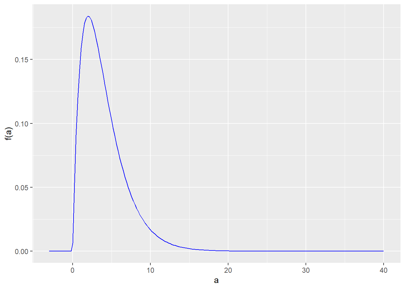
Based on these figures:
- Is \(x\) discrete or continuous?
- Which graph shows the PDF and which graph shows the CDF?
- Approximately what value is the median of \(x\)?
- Is \(x\) more likely to be between 0 and 10, or between 10 and 20?
GOAL #2: Know and use the key properties of the uniform distribution
- Suppose that \(x \sim U(-1,1)\).
- Find the PDF \(f_x(\cdot)\) of \(x\).
- Find the CDF \(F_x(\cdot)\) of \(x\).
- Find \(\Pr(x = 0)\).
- Find \(\Pr(0 < x < 0.5)\).
- Find \(\Pr(0 \leq x \leq 0.5)\).
- Find the median of \(x\).
- Find the 75th percentile of \(x\).
- Find \(E(x)\).
- Find \(var(x)\).
GOAL #3: Derive the distribution for a linear function of a uniform random variable
- Suppose that \(x \sim U(-1,1)\), and let \(y = 3x + 5\).
- What is the probability distribution of \(y\)?
- Find \(E(y)\).
GOAL #4: Know and use the key properties of the normal distribution
- Suppose that \(x \sim N(10,4)\).
- Find \(E(x)\).
- Find the median of \(x\).
- Find \(var(x)\).
- Find \(sd(x)\).
- Use Excel to find \(\Pr(x \leq 11)\).
GOAL #5: Derive the distribution for a linear function of a normal random variable
- Suppose that \(x \sim N(10,4)\).
- Find the distribution of \(y = 3x + 5\).
- Find a random variable \(z\) that is a linear function of \(x\) and has the standard normal distribution.
- Find an expression for \(\Pr(x \leq 11)\) in terms of the standard normal CDF \(\Phi(\cdot)\).
- Use the Excel function
NORM.S.DISTand the previous result to find to find the value of \(\Pr(x \leq 11)\).
GOAL #6: Derive the joint PDF of two discrete random variables from the probability distribution of a random outcome
- Let \(f_{y,b}(\cdot)\) be the joint PDF of \(y\) and \(b\), where \(y\) is an
indicator for winning a “Yo” bet in craps, and \(b\) is an indicator for
winning a “Boxcars” bet.
- Find \(f_{y,b}(1,1)\).
- Find \(f_{y,b}(0,1)\).
- Find \(f_{y,b}(1,0)\).
- Find \(f_{y,b}(0,0)\).
GOAL #7: Calculate a marginal PDF from a (discrete) joint PDF
- Let \(f_b(\cdot)\) be the marginal PDF of \(b\), where \(b\) is an indicator for
winning a “Boxcars” bet in craps.
- Find \(f_b(0)\) based on the joint PDF \(f_{y,b}(\cdot)\).
- Find \(f_b(1)\) based on the joint PDF \(f_{y,b}(\cdot)\).
- Find \(E(b)\) based on this marginal PDF you found in parts (a) and (b).
GOAL #8: Derive a conditional PDF from a (discrete) joint PDF
- Let \(f_{y|b}(1,1)\) be the conditional PDF of \(y\) given \(b\), where \(y\) is an
indicator for winning a “Yo” bet in craps, and \(b\) is an indicator for
winning a “Boxcars” bet.
- Find \(f_{y|b}(1,1)\).
- Find \(f_{y|b}(0,1)\).
- Find \(f_{y|b}(1,0)\).
- Find \(f_{y|b}(0,0)\).
GOAL #9: Interpret joint, marginal, and conditional distributions
- You have bet on Yo and your friend Betty bet on Boxcars. Based on your
previous calculations:
- What is the probability you and Betty both win?
- What is the probability you and Betty both lose?
- What is the probability Betty wins?
- What is the probability that you win if Betty loses?
GOAL #10: Determine whether two random variables are independent
- Which of the following pairs of random variables are independent for a
single game of craps?
- \(y\) and \(t\)
- \(y\) and \(b\)
- \(r\) and \(w\)
- \(r\) and \(y\)
GOAL #11: Calculate the covariance of two discrete random variables from their joint PDF
- Find \(cov(y,b)\) using the joint PDF \(f_{y,b}(\cdot)\) calculated in problem
- above.
GOAL #12: Calculate the covariance of two random variables using the expected value formula
- Find the following covariances using the alternate formula, where \(y\) is an
indicator for winning a “Yo” bet in craps, and \(b\) is an indicator for
winning a “Boxcars” bet.
- Find \(E(yb)\) using the joint PDF \(f_{y,b}(\cdot)\).
- Find \(cov(y,b)\) using your result in (a).
- Is your answer in (b) the same as your answer to question 5 above?
GOAL #13: Calculate the correlation of two random variables from their covariance
Find \(corr(y,b)\) using the results you found earlier, where \(y\) is an indicator for winning a “Yo” bet in craps, and \(b\) is an indicator for winning a “Boxcars” bet.
We can find the correlation from the covariance, but we can also find the covariance from the correlation. For example, suppose we already know that \[\begin{align} E(t) &= 7 \nonumber \\ var(t) &\approx 5.83 \nonumber \\ corr(b,t) &\approx 0.35 \nonumber \end{align}\] Using this information and the values of \(E(b)\) and \(var(b)\) implied by the fact that \(b \sim Bernoulli(1/36)\)
- Find \(cov(b,t)\).
- Find \(E(bt)\).
GOAL #14: Calculate the correlation and covariance of two independent random variables
- We earlier found that \(r\) and \(w\) (the values rolled on two separate dice)
are independent. Using this information:
- Find \(cov(r,w)\).
- Find \(corr(r,w)\).
GOAL #15: Calculate the expected value of a linear function of two or more random variables
- Your net winnings if you bet $1 on Yo and $1 on Boxcars can be written
\(16y + 31b - 2\). Find the following expected values:
- Find \(E(y + b)\)
- Find \(E(16y + 31b - 2)\)
- Find the following variances and covariances,, where \(y\) is an indicator for
winning a “Yo” bet in craps, and \(b\) is an indicator for winning a “Boxcars”
bet.
- Find \(cov(16y,31b)\)
- Find \(var(y + b)\)
GOAL #16: Interpret covariances and correlations
- Based on your results, which of the following statements is correct?
- The result of a bet on Boxcars is positively related to the result of a bet on Yo.
- The result of a bet on Boxcars is negatively related to the result of a bet on Yo.
- The result of a bet on Boxcars is not related to the result of a bet on Yo.
if \(b <0\), then \(y \sim U(a + bH, a + bL)\).↩︎
More precisely, either or both of \(\sigma_x\) and \(\sigma_y\) could be zero. In that case the covariance will also be zero, and the correlation will be undefined (zero divided by zero).↩︎
More generally, \(corr(ax+b,cy+d) = sign(a)\,sign(b)\,corr(x,y)\) for any (positive or negative) constants \(a,b,c,d\).↩︎