Chapter 10 An introduction to R
As we have seen, Excel is a useful tool for both cleaning and analyzing data. R is an application that has many of the same features as Excel, but is specially designed for statistical analysis. It is a little more complex, but more powerful in many important ways.
This chapter will introduce you to some of the basic concepts of R and associated tools such as R Markdown, RStudio, and the Tidyverse.
Chapter goals
In this chapter, we will learn how to:
- Perform basic tasks in RStudio, including:
- Executing commands in the console window.
- Creating, opening, closing and executing scripts.
- Creating and kitting R Markdown documents.
- Describe and use R language elements, including:
- Expressions
- Variables
- Vectors
- Lists
- Attributes
- Functions and operators
- Install and load R packages.
- Import and view data in R.
To prepare for this chapter, please ensure that you have R and RStudio available on your computer. Refer to the installation instructions as needed.
In this course, we will only have time to learn a little bit about R, so my goal is not to give a comprehensive treatment. My goal here is primarily to introduce you to the terminology and concepts of R, and to show you a few applications where R outshines Excel. You will learn much more about R in ECON 333 and (if you take it) ECON 334.
10.1 A brief tour of RStudio
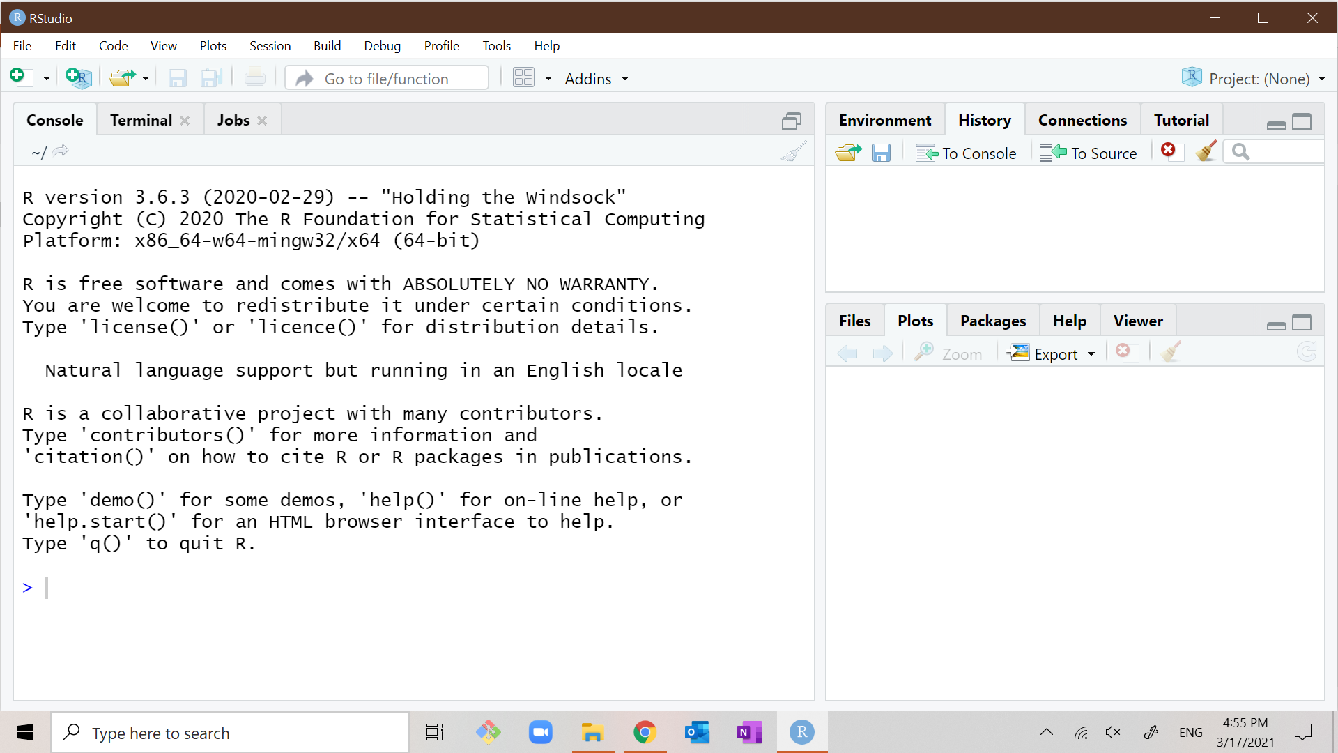
Start the program RStudio. You should see something that looks like this:
You may wonder what the difference is between R and RStudio. R is two
things:
- A programming language designed for statistical analysis
- A computer application that runs R commands.
RStudio is an integrated development environment (IDE) for R. It combines a set of useful tools for writing and running R code:
- An interactive session of the R application (running in the “Console” window).
- A text editor for writing R code, with features like syntax highlighting, spell check, and command auto-complete.
- Tools for managing files and packages used by R
- Tools for comparing and combining scripts and other files
- Help and documentation
- many other features
and puts them in a single user-friendly interface.
You can run commands and scripts in R itself, but without RStudio you won’t have these extra features. Most people these days use RStudio or another IDE.
RStudio normally displays three or four open windows, each of which has tabs you can select to access different features. We will not use most of them, but some of them will be very handy indeed.
R or Python?
The general-purpose programming language Python is a popular alternative to R for serious statistical analysis. Python is also available at no cost, and has some important advantages over R:
- Python is a general purpose programming language and is more widely used for applications other than data cleaning and analysis.
- Cutting-edge data science and machine learning tools are typically developed in Python, though most are also available in R.
- Because of this, Python skills look better on your resume.
So why are we learning R?
- Using Python for even the most basic data cleaning and analysis requires the user to install and maintain various external packages: NumPy for math, Pandas for data management, and Matplotlib for graphs. These capabilities are built into R.
- Configuring your Python installation and managing external packages can be complex, and can distract
My own experience is that the specific programming language you learn is not particularly important. I have written code in R, Python, Fortran, Stata, Basic, VBA, Pascal, assembly language, Gauss, Perl, SHAZAM, and EViews. Every language has its distinctive features, but translating from one language to another is usually easy if you have command of concepts like control flow statements (if-then branching, do-loops), functions, operators, array indexing, vector mathematics, data types, etc.
My advice is to focus on building language-independent skills, and plan to take an introductory computer science course where you learn Python as a general-purpose language. Your experience with R will help you in that course, and your knowledge of R as a statistical package and Python as a language will prepare you well to use Python in data analysis.
10.1.1 The console window
Like most programming languages, R is designed to execute a series of commands provided by the user. The simplest way to have R execute a command is by entering it into the Console window in the lower left corner.
Example 10.1 Using the console window
Move your cursor into the console window, type this command:
and press the <Enter> key. R will respond with something like:
## [1] "Hello world!"You have just executed your first R command.
The rest of this chapter will show you various R commands, and will display the expected results. Note that:
- Commands and results will be displayed in a single block.
- Lines with results will start with
##.
You can copy any block of R code from the web page version of this textbook by
clicking in the upper right-hand corner of the block. You can then paste the
block into the console window, and hit the <Enter> key. Give this trick a try
with the block above; you will find it handy whens the commands are longer and
more complex.
RStudio has various features to make your work in the console window more efficient:
- RStudio will offer to auto-complete your command.
- RStudio shows pop-ups with helpful information about your command as you type it.
- RStudio maintains a command history that remembers commands you have previously entered.
The command history can be quite useful when you did something a while ago, but either don’t remember exactly how you did it, or don’t want to type it all in from the beginning.
Example 10.2 Using the command history
Suppose you decide you want to say “Hello Canada!” instead of “Hello world”, and you don’t want to type in the whole command. Then you can:
- Press the
<Up-arrow>key in the Console window to show the most recently executed command. If you press it a second time it gives you the command before that, and so on. - Look at the to the History window in the upper right corner to see a full list of recently executed commands. You can double-click on any command in the window to copy it to the Console window.
Once you have found the command you want, you can edit it before pressing the
<Enter> key.
10.1.2 Scripts
The Console window is ideal for simple tasks and experimentation, and we will
continue using it regularly. But in order to create reproducible research and
take full advantage of R’s capabilities, we will need to write and execute
scripts. A script is just a text file containing a sequence of R commands.
By convention, R scripts have file names ending in the .R extension.
Example 10.3 Using an R script
To create an R script
Select
File > New File > R Scriptfrom the menu.Enter a valid R command in the first line of the file, for example
Enter another valid R command in the second line of the file, for example
Select
File > Saveto save your file with the nameChapter10Example.R.
To run your script:
- Press the
 button.
The Console window will show the results of your script:
## [1] "Hello world!"
## [1] "Goodbye world?"
In addition to the Source button, there is another button marked Run.
Pressing this button will run the script one line at a time.
10.1.3 R Markdown
RStudio can also run text files written in the R Markdown format. R
Markdown files have the .Rmd extension. R Markdown is a language for
producing documents - web pages, Microsoft Word documents,
PDF files, etc. - that have R code and analysis embedded in them. In fact, this
book is written in R Markdown - you can see the R Markdown document for this
chapter at https://raw.githubusercontent.com/bvkrauth/is4e/master/10-Introduction-to-R.Rmd.
R Markdown, Markdown, and other markup languages
R Markdown is an implementation of the Markdown markup language in R. A markup language is a way of writing documents in text files whose content is directly readable but also can be formatted and displayed (rendered) in a visually appealing way. The best-known markup language is HTML, which is the language web pages are written in.
The original idea of HTML was that content creators could write their content in text files (pages), with a few HTML tags sprinkled around to give the browser information about structure, and then the browser would display the page. However, as web users demanded fancy graphics, custom colors, interactivity, and mobile-friendly display, HTML became much more complicated.
Markdown was created as radically simplified markup language. The basic idea is to use common conventions for how to indicate structure in a text file.
- Adjacent lines of text are interpreted as part of the same paragraph.
- A line of text following a blank line starts a new paragraph.
- A line of text that begins with “#” is a header, with “#” for level one headers, “##” for level two, etc.
- A line of text that begins with “-” is a bullet point.
- A line of text that begins with a number is part of a numbered list.
- Text written like
*this*is rendered like this. - Text written like
**this**is rendered like this. - Text written like
***this***is rendered like this.
Markdown documents can also include links and pictures (by simply providing the URL or file name), tables, and all sorts of other things.
In addition to ordinary text and Markdown information, R Markdown documents can include pieces of executable R code. R code needs to be surrounded by a code fence that identifies the text inside the fence as R code, and in some cases provides additional information about how it should be executed. This might sound complicated, but is easy to see in a real R Markdown file.
Example 10.4 Creating an R Markdown file
To create our first R Markdown file:
- Select
File > New File > R Markdownfrom the menu.- You will see a dialog box that looks like this:
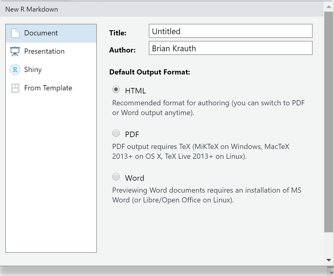
- You will see a dialog box that looks like this:
- The default options are fine, so select
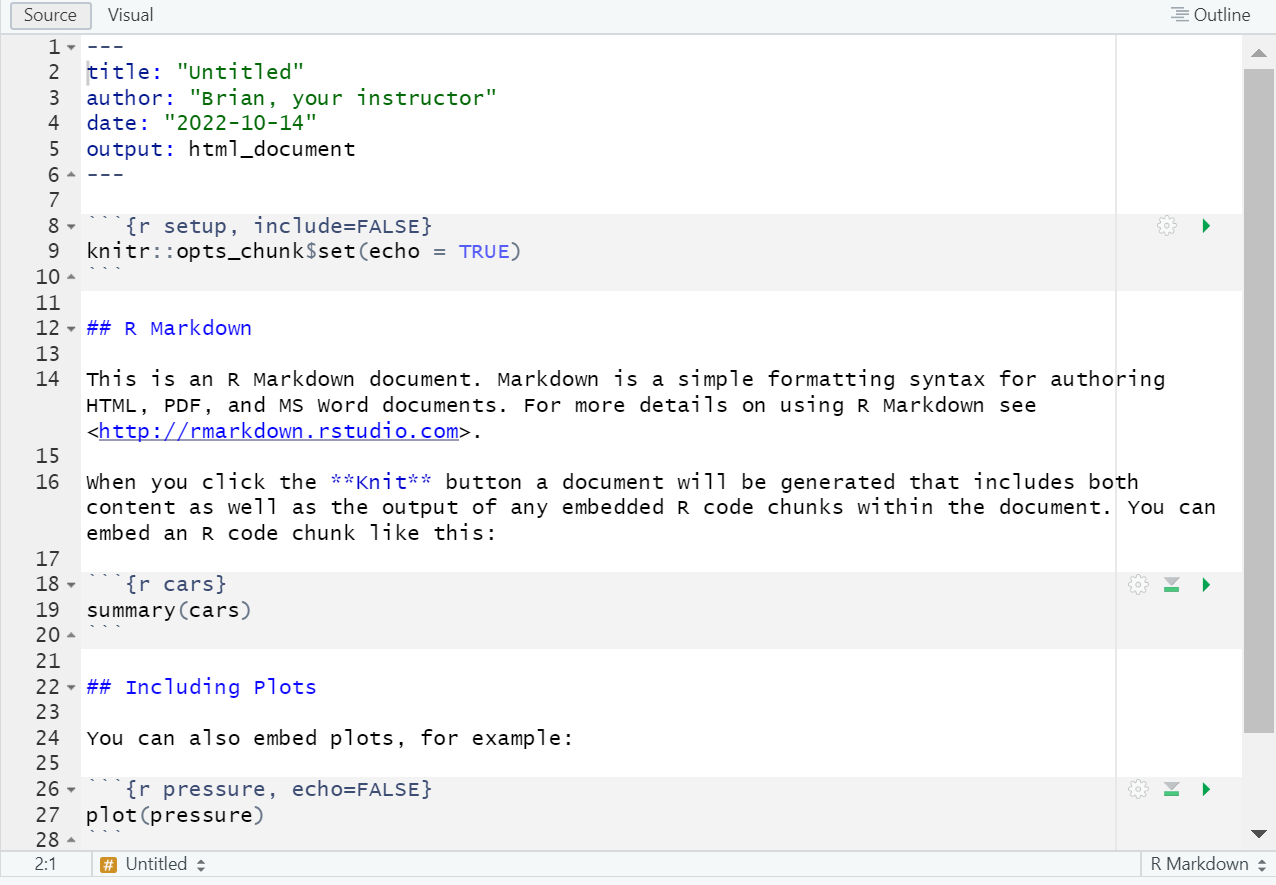
OK. RStudio will create an example R Markdown file that you can use as a template. It will look something like this:
- Save the file.
You can see that the R Markdown document is a mix of text, formatting information, and small pieces of R code.
You can run the R code in an R Markdown document in one of two ways. First, you can run and display results for individual chunks of code. A chunk is a few lines of R code surrounded by a “code fence” that serves to distinguish R code from ordinary text.
Example 10.5 Running code chunks
To run a code chunk in our R Markdown file:
- Go to the code chunk that looks like this:
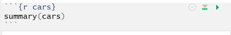
- Press the
 button.
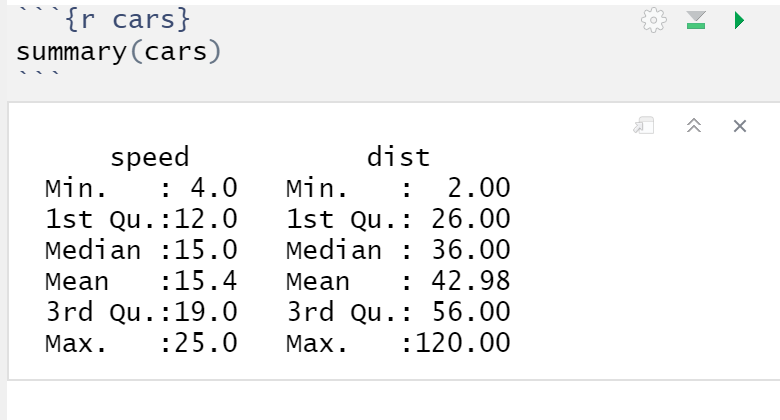
As you can see, the code in the chunk will run and the results will be displayed
below:
You can also press the Knit button to knit the entire R Markdown file into an HTML, Word, or PDF document that includes both the text and the R results.
Example 10.6 Knitting an R Markdown document
To knit the entire document into a web page:
- Press the
 button.
It will take a few moments to process the file, and then the web page (HTML file) will open in a browser. Read the document and compare it to the original R Markdown file to get an idea of the capabilities of R Markdown.
By default, R Markdown files usually knit to HTML, but we can knit to other file formats including Word and PDF. We will stick to HTML in this course.
R Markdown resources
R Markdown is as simple or as complicated as you want to make it. A plain text file with a few lines of content is a valid R Markdown file even if it contains no R code. You can knit it, and R will produce a valid web page or other document for you.
If you want to try something new in R Markdown, or have forgotten how to do something, the most useful resource is the one-page R Markdown Cheat sheet. It is available directly in RStudio, or at https://github.com/rstudio/cheatsheets/raw/main/rmarkdown-2.0.pdf. You can also just search for “r markdown cheatsheet”.
10.1.4 Other RStudio features
RStudio has many other features, most of which we will not use. But I would like to highlight a few that may seem useful.
In the lower right window:
- The Files tab gives you easy access to files in the current active folder.
- The Plots tab will display plots, when you create them.
- The Packages tab is useful for managing packages (more on them later)
- The Help tab allows you to access R’s help system.
In the upper right window:
- The Environment tab allows you to view all currently-defined variables and their values.
- The History tab shows the command history.
In the menu:
- You can select
Session > Restart Rto clear the memory and restart the current R session.
Never save your workspace
I would also like to highlight a “feature” that is not at all useful and should
be avoided. When you close R or RStudio, you may get a warning message
that looks something like this:
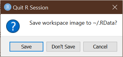
If you choose “Save”, R will save the current state of its memory and re-load it next time you start R. This may seem like it would be helpful, but it is actually bad. We care about reproducibility, so we want R to do exactly the same thing every time we use it. We do not want R’s actions to depend on something we did a few days ago. So NEVER CHOOSE “Save” HERE.
10.2 The R language
Next, we will learn some basic features of the R language. Learning a programming language is a lot like learning a regular language: it helps to know the rules, but you need to learn by doing.
Each of the subsections in this section goes through a particular element of the R language. As you go through each subsection, my recommendation is to:
- Try out all of the examples.
- If you aren’t sure exactly how something works, modify the example to see what happens. Keep doing this until you understand.
- Once you understand something, move on to the next subsection.
Open RStudio and go to the console window.
10.2.2 Expressions
An expression is any piece of R code that can be evaluated on its own. For example:
- Any text, numerical or logical constant:
"Hello world",105,1.34, orTRUE. - Any complete formula built from functions and arithmetic operators:
log(10)or2+2
An expression needs to be complete, for example ln( is not an expression, nor
is 2+.
Every valid R expression returns a value, also called an object. For example:
- The expression
"Hello world"returns the text string “Hello world” - The expression
2+2returns the number 4.
An object can be a number, a text string, a date, or a logical value, just like in Excel. Objects can also be much more complex.
In addition, some expressions cause a side effect. For example, executing an expression may cause R to:
- Display something on your screen.
- Create or modify a file on your computer.
- Create or modify an object in R’s memory.
For example, the expression print("Hello world") returns the value
“Hello world” and (as a side effect) causes
## [1] "Hello world!"to be displayed on your screen.
Any valid R expression can be entered in the console window, in an R script, or in an R Markdown document.
Example 10.8 Expressions
When you enter an expression in the console window, R will usually display the value it returns.
You can also use any valid R expression within a larger expression.
This expression has a side effect. It causes R to plot a histogram of 100 random numbers from the \(N(0,1)\) distribution.
Although we call it a “side effect”, the side effect is often the main purpose of the expression.
10.2.3 Variables and assignment
We can use the <- or assignment operator to assign the result of an
expression to a named variable. We can then use that variable in later
expressions.
For example, the R command x <- 2 assigns the value 2 to the variable x.
Any subsequent code can then refer to the variable x in its own calculations
or actions.
Example 10.9 Using the assignment operator
We can display the contents of a variable or other object by using the print()
function, or by simply giving its name
10.2.4 Vectors
The primary data structure in R is a vector, which is just an ordered list of elements.
The simplest type of vector is called an atomic vector - its elements are normally from one of R’s basic or atomic data types:
- Numbers
- Text strings
- Logical values (
TRUEorFALSE)
The elements of an atomic vector need to be all part of the same atomic type; a single vector cannot contain both strings and numbers, for example.
We can construct a vector by enumeration using the c() function.
Example 10.11 Constructing a vector with the c() function
There are many other functions that can be used to construct vectors. Two
particularly useful ones are rep which repeats something a particular number
of times, and seq which creates a sequence.
Example 10.12 Constructing vectors with rep() and seq()
# REP repeats something (like Excel's Fill tool)
ones <- rep(1, times = 10)
print(ones)
##  [1] 1 1 1 1 1 1 1 1 1 1
# SEQ creates a sequence (like Excel's Series tool)
evens <- seq(from = 2, to = 20, by = 2)
print(evens)
##  [1]  2  4  6  8 10 12 14 16 18 20
# You can also create a sequence with the : operator:
print(1:10)
##  [1]  1  2  3  4  5  6  7  8  9 10
Mathematical functions in R operate directly on vectors, and automatically expand scalars (single numbers) to vectors as needed.
Example 10.13 Using vectors in expressions
The subscript operator [] can be used to select part of a vector.
Example 10.14 Using subscripts
evens <- seq(from = 2, to = 20, by = 2)
print(evens)
##  [1]  2  4  6  8 10 12 14 16 18 20
# You can give a single index: evens[2] is the 2nd element in evens
x <- evens[2]
print(x)
## [1] 4
# Or a vector of indices: evens[c(2,5)] contains the 2nd and 5th element in evens
x <- evens[ c(2, 5) ]
print(x)
## [1]  4 10
# Or a range of indices: evens[2:5] contains 2nd, 3rd, 4th and 5th element in evens
x <- evens[2:5]
print(x)
## [1]  4  6  8 10
# You can use the subscript operator on either side of the assignment operator
x <- evens
print(x)
##  [1]  2  4  6  8 10 12 14 16 18 20
# This assigns the number 1000 to the 2nd element in x
x[2] <- 1000
print(x)
##  [1]    2 1000    6    8   10   12   14   16   18   20
You can also provide logical values as subscripts. R will then operate on those
elements whose corresponding item has the value TRUE.
Example 10.15 Using logical subscripts
print(evens)
##  [1]  2  4  6  8 10 12 14 16 18 20
# This creates a vector of the same length as evens, that contains TRUE
# for all values less than 10, and FALSE for all other values
lessthan10 <- (evens < 10)
print(lessthan10)
##  [1]  TRUE  TRUE  TRUE  TRUE FALSE FALSE FALSE FALSE FALSE FALSE
# This creates a vector that includes only those elements of evens
# for which forexample is TRUE
x <- evens[lessthan10]
print(x)
## [1] 2 4 6 8
# This is a quicker way of accomplishing the same result
x <- evens[evens < 10]
print(x)
## [1] 2 4 6 8
10.2.5 Lists
The other type of vector is a list. A list is a vector whose elements are themselves other vectors. These vectors can be any type, so we can use lists inside lists to build very complex objects.
Lists can be built using the list() function.
Example 10.16 Constructing a list
You can (and should) assign names to the elements of a list.
Example 10.17 Constructing a named list
You can access part of a list by specifying its numerical index inside of the
[[]] operator.
If the items in a list are named, you can also access them by name using either
[[]] or $ notation. You can also use the $ notation to add new items to
an existing list.
Example 10.19 Selecting parts of a named list
We can access the elements of a list by name:
print( everything[["evens"]] )
##  [1]  2  4  6  8 10 12 14 16 18 20
print( everything$fruits )
## [1] "Avocado"    "Banana"     "Cantaloupe"
And we can add named elements:
# There is no element in everything called "allnumbers"
everything$allnumbers <- c(evens, odds)
# But now there is...
print(everything)
## $fruits
## [1] "Avocado"    "Banana"     "Cantaloupe"
##
## $evens
##  [1]  2  4  6  8 10 12 14 16 18 20
##
## $odds
##  [1]  1  3  5  7  9 11 13 15 17 19
##
## $allnumbers
##  [1]  2  4  6  8 10 12 14 16 18 20  1  3  5  7  9 11 13 15 17 19
10.2.6 Functions and operators
R has hundreds of built-in mathematical and statistical functions, and users can define their own functions. You have already seen a few. Their format and usage is quite similar to Excel, but there are some important differences.
Example 10.20 The seq() function
Let’s get to know the main features of functions in R by considering the
seq() function. We have already seen this function: it is used to create a
vector with a sequence of numbers, much like Excel’s Series tool.
Every function has a name.
- In this case, the function’s name is
seq.
- In this case, the function’s name is
You can obtain help on any function by entering
?and its name in the console window- Enter
? seqin the console window, and look in the Help window (you can find it in the lower-right panel).
- Enter
Most functions accept one or more arguments.
- The arguments are described in the function’s help page.
- The
seqfunction’s arguments includefrom,to,by,length.out, andalong.with. - Every argument has a name and a position. For example, the
fromargument is in position one, thetoargument is in position two, etc. - Arguments can be passed to the function by name or by position.
- Passing by name looks like this:
seq(from=1,to=5). - Passing by position looks like this:
seq(1,5). - You can mix both methods:
seq(1,5,length.out=10). - I recommend passing by position for simple functions, and passing by name for more complex functions, but it is really just a matter of what works for you.
- Passing by name looks like this:
- Some arguments are required. They must be provided every time the function is called, or else the function will return an error.
- Some arguments are optional. They can be provided, but have a default
value if not provided.
- All arguments to
seq()are optional; execute the commandseq()to see what happens.
- All arguments to
Every function returns a value. This is even true for functions like
print(). To see this:As you can see,
print("Hello world")returns “Hello world” as its value.Some functions also produce side effects, as we have described earlier.
In addition to functions, R has the usual binary mathematical operators
such as +, -, * and /. Operators are just another way of expressing
functions. For example the + operator is really just another way of calling
the sum() function:
There are several other commonly used operators including comparison operators, logical operators, and the assignment operator.
Example 10.21 A few useful operators
# Basic arithmetic operators
2 + 3 # plus
## [1] 5
2 - 3 # minus
## [1] -1
2 * 3 # times
## [1] 6
2 / 3 # division
## [1] 0.6666667
2 ^ 3 # power
## [1] 8
# Comparison operators
2 < 3  # less than
## [1] TRUE
2 <= 3 # less than or equal
## [1] TRUE
2 == 3 # equal
## [1] FALSE
2 > 3  # greater than
## [1] FALSE
2 >= 3 # greater than or equal
## [1] FALSE
# Logical operators
2 == 3 & 2 < 3 # logical AND
## [1] FALSE
2 == 3 | 2 < 3 # logical OR
## [1] TRUE
# Assignment
x <- 2
print(x)
## [1] 2
# The assign() function returns its own value, so you can also do this:
x <- y <- 3
print(x)
## [1] 3
print(y)
## [1] 3
10.2.7 Classes and attributes
Classes and attributes are something of an advanced topic, but we will briefly mention them here.
Every object in R has a class, which is just a text string identifying
what kind of thing it is. The class of any object can be accessed using
the class() function
Example 10.22 Classes
The class of an object tells R how to handle it - how to display or summarize its contents, how to use it in functions, etc. R has hundreds of built-in classes, including:
- Matrices.
- Arrays.
- Data sets.
- Statistical results from various commands.
- Plots.
These object types are all built from basic components like atomic vectors and lists. Users can also define their own classes.
Classes and object oriented programming
Classes appear in most modern programming languages, and are a key component of the “object-oriented” programming model. OOP allows programmers to design very complicated data structures that are also easy to use.
For example, a novice user like yourself can display the contents of any object
using the print() function and can get a brief summary of those contents using
the summary() function. This works with simple objects like “Hello world”
or more complex objects like a large data set, a graph of results, or a machine
learning model.
Underlying this simple user interface, print() is a generic function that
takes any object, determines its class, and then calls a specific print
function that is specially designed for its class. Programmers create both
the class design and the associated specialized functions. Normal users only
need to know the print() function.
Objects can also have attributes. The attributes of an object are a list that provides additional information about the object.
Example 10.23 Attributes
Let’s see if any of the objects we have created have attributes:
print(attributes(fruits))
## NULL
print(attributes(evens))
## NULL
print(attributes(everything))
## $names
## [1] "fruits"     "evens"      "odds"       "allnumbers"
Note that:
- our two atomic vectors (
fruitsandevens) have no attributes (NULL). - our list (
everything) stores the names of its three elements in the$namesattribute.
10.3 Packages and the Tidyverse
R has many useful built-in functions and features. But one of its most useful features is how easily it can be extended by users, and the fact that it has a large user community who have provided packages of useful new functions and data.
There are thousands of packages available online. We will use a popular and useful package called the Tidyverse.
What is the Tidyverse?
The Tidyverse was created by the data scientist Hadley Wickham (also one of the key people behind RStudio) as a way of solving some long-standing problems with R. The Tidyverse is both an R package containing a set of new functions and data structures as well as a philosophy about how to analyze data.
The main language elements of R date back to 1976 (R itself was created in the early 1990s but is closely based on an earlier program called S). Computer science has advanced a lot since 1976, so some design aspects of R seemed like a good idea at the time but would be designed differently today:
- Too many different ways of doing the same thing.
- Too many rarely-used functions.
- Some functions that don’t do what they should.
Unfortunately, it is not possible to make significant changes to the existing R language (sometimes called “Base R”) without causing thousands of existing programs to stop working.
The Tidyverse addresses this problem by replacing many Base R functions with alternative versions that are easier to use, better-designed, and usually faster. It does this in part by being “opinionated” - taking a clear position on the right way to do things and building the language around this position. For example, most data analysis tools in the Tidyverse expect data to be in a tidy format. This reflects a philosophy that data cleaning should precede and be separate from data analysis.
Most commonly-used packages including the Tidyverse are open-source, and are available online from the Comprehensive R Archive Network (CRAN).
Before you can use any package, two steps must be followed:
- Install the package on your computer using the
install.packages()function.- This only needs to be done once for each package.
- Load the package into memory using the
library()function.- This needs to be done in every R session in which the package is used.
Once the package is installed and loaded, you can use its functions and other features.
Example 10.24 Installing and loading the Tidyverse
You can get a list of all available CRAN packages by simply executing the
install.packages() function with no arguments:
If you know the name of the CRAN package you want to install, you can provide it as the argument:
You only need to install each package once.
However, installing a package only puts the files on your computer. In order to
actually use the features of a package you need to load it into memory during
your current R session using the library() function:
You can then use the Tidyverse functions and other tools.
10.4 Reading and viewing data in R
Having skimmed the basic features of R, it is time to use it for some real work. As with Excel, we start any data analysis project in R by opening the data file, viewing it, and constructing a plan to clean it.
We will work with the employment data.
10.4.1 Reading a CSV file
Our first step will be reading the data. The most commonly used data format is
CSV, and the Tidyverse function to read in CSV files is called read_csv().
It has one required argument: the name of the CSV file, either as a local file
address or a URL. It returns an object called a data table or tibble.
A tibble is a Tidyverse object type that describes a table of tidy data.
- Each row in the tibble represents an observation.
- Each column represents a variable, and has a name.
As a side effect, read_csv() also displays information about the tibble it
has created.
Example 10.25 Reading a CSV file in R
The code below reads in the CSV file, and stores it in the object EmpData.
# Load the Tidyverse if you have not already done so
library("tidyverse")
# You can directly read online data by giving read_csv() the URL.
EmpData <- read_csv("https://bookdown.org/bkrauth/IS4E/sampledata/EmploymentData.csv")
# You can also download the file and give read_csv() the local location
# EmpData <- read_csv("sampledata/EmploymentData.csv")
## Rows: 541 Columns: 11
## ── Column specification ──────
## Delimiter: ","
## chr (3): MonthYr, Party, PrimeMinister
## dbl (8): Population, Employed, Unemployed, LabourForce, NotInLabourForce, Un...
##
## ℹ Use `spec()` to retrieve the full column specification for this data.
## ℹ Specify the column types or set `show_col_types = FALSE` to quiet this message.As you can see from the information displayed, R guesses each column’s data type, and reports its guess. The guesses are usually good, but you can override them if not. It is always a good idea to review this output and make sure that everything is the way that we want it:
- The numeric variables are all stored as
col_double().- This means double-precision (64 bit) real number.
- This is what we want.
- The text variables Party and PrimeMinister are both stored as
col_character().- This means character or text string.
- This is what we want.
- The MonthYr variable is also stored as
col_character().- This is not what we want.
- We will want MonthYr to be stored explicitly as a date variable.
We make a note of the issue with the MonthYr variable so we can fix it later.
Additional options
Our data file happens to be a nice and tidy one, so read_csv() worked just
fine with its default options. Not all data files are so tidy, so read_csv()
has many optional arguments. There are also functions for other delimited file
types:
read_csv2()for files delimited by semicolons rather than commas.read_tsv()for tab-delimited files.read_delim()for files delimited using any other character.
Base R has a similar function called read.csv(), but the Tidyverse function read_csv() is preferable for various reasons.
10.4.2 Viewing a data table
We have several ways of viewing the contents of a tibble. As with other objects,
we can use the print() function.
Example 10.26 Printing a tibble
The code below prints the contents of our data table:
print(EmpData)
## # A tibble: 541 × 11
##    MonthYr Population Employed Unemployed LabourForce NotInLabourForce UnempRate
##    <chr>        <dbl>    <dbl>      <dbl>       <dbl>            <dbl>     <dbl>
##  1 1/1/19…     16852.    9637.       733       10370.            6483.    0.0707
##  2 2/1/19…     16892     9660.       730       10390.            6502.    0.0703
##  3 3/1/19…     16931.    9704.       692.      10396.            6535     0.0665
##  4 4/1/19…     16969.    9738.       713.      10451.            6518.    0.0682
##  5 5/1/19…     17008.    9726.       720       10446.            6562     0.0689
##  6 6/1/19…     17047.    9748.       721.      10470.            6577.    0.0689
##  7 7/1/19…     17086.    9760.       780.      10539.            6546.    0.0740
##  8 8/1/19…     17124.    9780.       744.      10524.            6600.    0.0707
##  9 9/1/19…     17154.    9795.       737.      10532.            6622.    0.0699
## 10 10/1/1…     17183.    9782.       783.      10565.            6618.    0.0741
## # ℹ 531 more rows
## # ℹ 4 more variables: LFPRate <dbl>, Party <chr>, PrimeMinister <chr>,
## #   AnnPopGrowth <dbl>
Tibbles can be quite large, so the print() function usually shows an
abbreviated version of the table. We can also see the whole table by using
the View() command or through RStudio.
Example 10.27 Viewing a tibble
You can view the full tibble by executing the command:
View(EmpData)or through RStudio by following these steps:
- Go to the Environment tab in the upper right window.
- You will see a list of all variables currently in memory, including EmpData.
- Double-click on
EmpData.
You will see a spreadsheet-like display of EmpData. As in Excel, you can sort
and filter this table. Unlike Excel, you cannot edit it here.
10.4.3 Data table properties
The base R equivalent of a tibble is called a data frame. Tibbles and data frames are interchangeable in most applications (in the language of object-oriented programming, the tibble class “inherits” from the data frame class), but tibbles have some additional features that make them work better with the Tidyverse.
There are several R functions available for exploring the properties of a data table.
- We can obtain the column names of a tibble using the
names()function. - We can access any individual column using the
$notation. - We can count the rows and columns with
nrow()andncol(), or we can use thelength()function.
These functions will also work with data frames.
Example 10.28 Viewing properties of a tibble
# Column names
names(EmpData)
##  [1] "MonthYr"          "Population"       "Employed"         "Unemployed"
##  [5] "LabourForce"      "NotInLabourForce" "UnempRate"        "LFPRate"
##  [9] "Party"            "PrimeMinister"    "AnnPopGrowth"
# Number of rows - either of these will work
nrow(EmpData)
## [1] 541
length(EmpData$UnempRate)
## [1] 541
# Number of columns
ncol(EmpData)
## [1] 11
length(EmpData)
## [1] 11
10.5 Basic statistics in R
Next we will learn a few simple commands for producing univariate summary statistics and graphs. We will expand on these commands in Chapter 11.
Before getting started, run the following code to clean the employment data:
# Clean EmpData
EmpData <- EmpData %>%
  mutate(MonthYr = as.Date(MonthYr, "%m/%d/%Y")) %>%
  mutate(UnempPct = 100*UnempRate) %>%
  mutate(LFPPct = 100*LFPRate)
Section 11.1 in Chapter 11 will discuss data cleaning in more detail, and will derive this block of code.
10.5.1 The summary function
The summary()function can be used to produce a set of summary statistics for
each variable in a tibble.
Example 10.29 Summarizing a data table
summary(EmpData)
##     MonthYr             Population       Employed       Unemployed
##  Min.   :1976-01-01   Min.   :16852   Min.   : 9637   Min.   : 691.5
##  1st Qu.:1987-04-01   1st Qu.:20290   1st Qu.:12230   1st Qu.:1102.5
##  Median :1998-07-01   Median :23529   Median :14064   Median :1265.5
##  Mean   :1998-07-01   Mean   :23795   Mean   :14383   Mean   :1261.0
##  3rd Qu.:2009-10-01   3rd Qu.:27327   3rd Qu.:16926   3rd Qu.:1404.6
##  Max.   :2021-01-01   Max.   :31191   Max.   :19130   Max.   :2609.8
##
##   LabourForce    NotInLabourForce   UnempRate          LFPRate
##  Min.   :10370   Min.   : 6483    Min.   :0.05446   Min.   :0.5996
##  1st Qu.:13467   1st Qu.: 6842    1st Qu.:0.07032   1st Qu.:0.6501
##  Median :15333   Median : 8162    Median :0.07691   Median :0.6573
##  Mean   :15644   Mean   : 8151    Mean   :0.08207   Mean   :0.6564
##  3rd Qu.:18230   3rd Qu.: 9099    3rd Qu.:0.09369   3rd Qu.:0.6674
##  Max.   :20316   Max.   :12409    Max.   :0.13697   Max.   :0.6766
##
##     Party           PrimeMinister       AnnPopGrowth         UnempPct
##  Length:541         Length:541         Min.   :0.007522   Min.   : 5.446
##  Class :character   Class :character   1st Qu.:0.012390   1st Qu.: 7.032
##  Mode  :character   Mode  :character   Median :0.013156   Median : 7.691
##                                        Mean   :0.013703   Mean   : 8.207
##                                        3rd Qu.:0.014286   3rd Qu.: 9.369
##                                        Max.   :0.024816   Max.   :13.697
##                                        NA's   :12
##      LFPPct
##  Min.   :59.96
##  1st Qu.:65.01
##  Median :65.73
##  Mean   :65.64
##  3rd Qu.:66.74
##  Max.   :67.66
##
Like print(), summary() is an example of a generic function. You can give it
almost any R object as an argument, and it will return a summary of the object’s
contents. The exact information returned will depend on the object type.
Section 11.2 in Chapter 11 will demonstrate additional R commands for univariate data analysis.
10.5.2 Introduction to ggplot
Although R has a built in plotting command called plot(), the Tidyverse also
contains a much more powerful graphics package called16
ggplot. The ggplot package has capabilities well beyond what R’s built-in
commands can do, or what Excel can do.
The ggplot function can be used to create a graph. It has a non-standard
syntax.
Example 10.30 Two ggplot graphs
We will use ggplot to create two univariate graphs for the unemployment rate: a time series (line) graph and a histogram. The variable representing the unemployment rate is called UnempPct and the variable representing the month/year is called MonthYr.
To make the time series (line) graph in Figure 10.1 below, execute the following code:
To make the histogram in Figure 10.2 below, execute the following code:
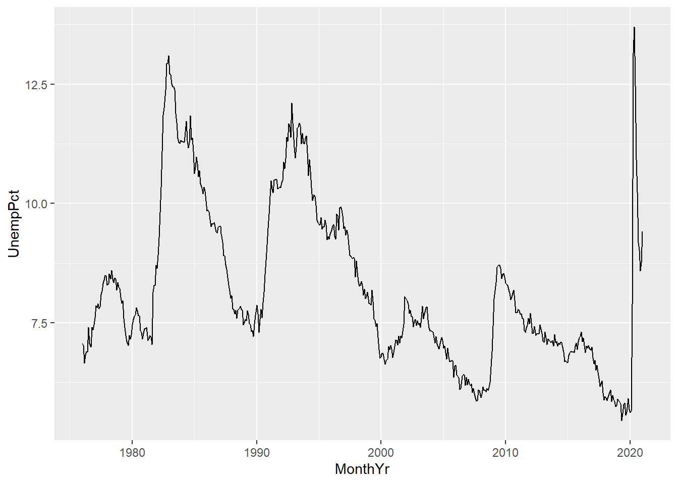
Figure 10.1: A time series graph created in ggplot
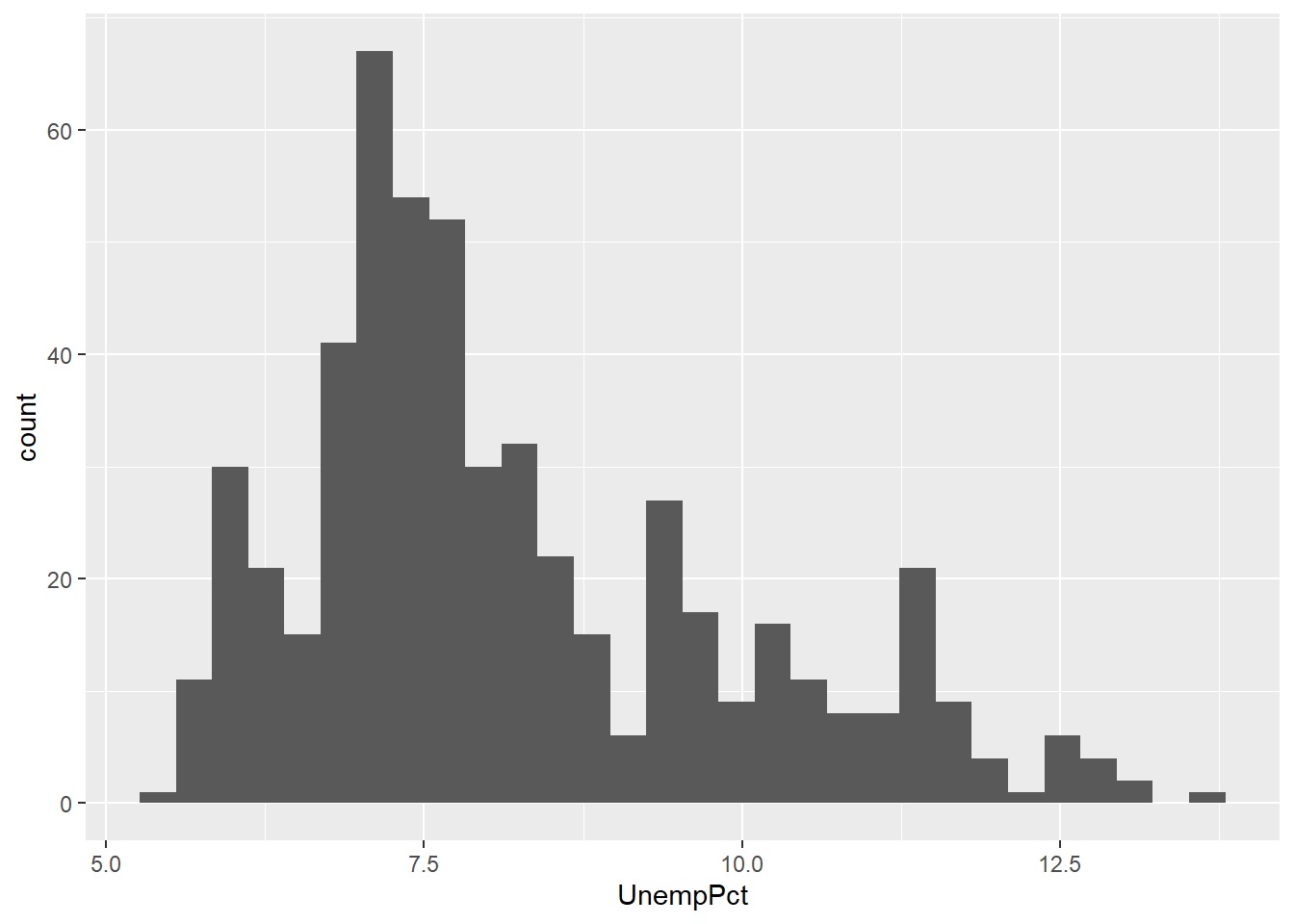
Figure 10.2: A histogram created in ggplot
Section 11.3 in Chapter 11 will explore ggplot and its capabilities in greater detail.
Chapter review
R has capabilities well beyond what you can do in Excel, in part because it is a full-featured language and not just an application. These capabilities come at a cost, which is that it takes more time and effort to learn how to do basic tasks. If you have little to no experience coding, this will take some extra effort but will be worth it. All languages commonly used for statistical analysis - R, Stata, SAS, Python, etc. - have more similarities than differences, and your experience using R will be useful regardless of what language you end up coding in later.
In this chapter, we learned how to run R programs whether in the console, in a script, or in an R Markdown document. We also learned the main elements of the R language, and a little bit of how to read and analyze data in R.
In the next chapter, we will learn to use R to clean, analyze and graph data. We will also learn some tools for visualization and prediction
For more information on R
There are many free sources of useful information about R.
- A good short introduction is available at https://cran.r-project.org/doc/contrib/Torfs+Brauer-Short-R-Intro.pdf.
- A good longer book that focuses on the Tidyverse is Wickham and Grolemund’s R for Data Science. It can be purchased as an actual book from Amazon or your local book shop, and is also available as a free e-book at https://r4ds.hadley.nz/.
Practice problems
Answers can be found in the appendix.
GOAL #1: Perform basic tasks in RStudio
- Open RStudio and do the following:
- Execute a command in the console window.
- Write and execute (source) a brief script.
- Write and knit a brief R Markdown document.
GOAL #2: Describe and use R language elements
- Which of the following are valid R expressions?
"Hello world"HelloHello"2+2x <- 2 + 2x <- 2 +
- Write the R code to perform the following actions:
- Create a vector named
cookiesthat contains the elements “oatmeal”, “chocolate chip”, and “shortbread”. - Create a vector named `
threesthat contains all of the integers between 1 and 100 that are divisible by 3. - Use the vector
threesto find the 5th-lowest integer between 1 and 100 that is divisible by 3. - Create a list named
threecookiesthat containscookiesandthrees.
- Create a vector named
GOAL #3: Install and load R packages
Load the tidyverse package (you will need to install it if you have not already done so), and execute the R code below:
data("mtcars")  # load data
ggplot(mtcars, aes(wt, mpg)) + geom_point(aes(colour=factor(cyl), size = qsec))
GOAL #4: Import and view data in R
- Use R (with the Tidyverse loaded) to open the data file https://people.sc.fsu.edu/~jburkardt/data/csv/deniro.csv and count the number of observations and variables in it.
The package is technically called
ggplot2since it is the second version ofggplot. But everyone calls it “ggplot” anyway.↩︎
10.2.1 Comments
In programming, a comment is a piece of code that is ignored by the program that interprets the code. Comments in R are marked by the
#character.Example 10.7 Comments
If you run the following code:
You will get the result:
Note that R treats the
#inside of the quotes as a normal character.Programmers use comments to explain to future users (including themselves) what the code is supposed to be doing.