Chapter 4 Random variables

Economics is a mostly quantitative field: its outcomes can be usually described using numbers: price, quantity, interest rates, unemployment rates, GDP, etc. Statistics is also a quantitative field: every statistic is a number calculated from data. When a random outcome is described by a number, we call that number a random variable. We can use probability theory to describe and model random variables.

This chapter will introduce the basic terminology and mathematical tools for working with simple random variables.

Chapter goals

In this chapter, we will learn how to:

Define a random variable in terms of a random outcome.
Determine the support and range of a random variable.
Calculate and interpret the PDF of a discrete random variable.
Calculate and interpret the CDF of a discrete random variable.
Calculate interval probabilities from the CDF.
Calculate the expected value of a discrete random variable from its PDF.
Calculate a quantile from the CDF.
Calculate the variance of a discrete random variable from its PDF.
Calculate the variance from expected values.
Calculate the standard deviation from the variance.
Calculate the expected value for a linear function of a random variable.
Calculate the variance and standard deviation for a linear function of a random variable.
Standardize a random variable.
Use standard discrete probability distributions:
- Bernoulli
- binomial
- discrete uniform.

To prepare for this chapter, please review the chapter on probability and random events and the section on sequences and summations in the math appendix.

4.1 Defining a random variable

A random variable is a number whose value depends on a random outcome. The idea here is that we are going to use a random variable to describe some (but not necessarily every) aspect of the outcome.

Example 4.1 Random variables in roulette

Here are a few random variables we could define in a roulette game:

The number the ball lands on: \[\begin{align} b = b(\omega) = \omega \end{align}\]
An indicator for whether a bet on red wins: \[\begin{align} r = r(\omega) = I(\omega \in RedWins) = \begin{cases} 1 & \textrm{if } \omega \in RedWins \\ 0 & \textrm{if } \omega \notin RedWins \\ \end{cases} \end{align}\]
The player’s net profits from $1 bet on red: \[\begin{align} y_{Red} = y_{Red}(\omega) = \begin{cases} 1 & \textrm{ if } \omega \in RedWins \\ -1 & \textrm{ if } \omega \in RedWins^c \end{cases} \end{align}\] That is, a player who bets $1 on red wins $1 if the ball lands on red and loses $1 if the ball lands anywhere else.
The player’s net profits from $1 bet on 14: \[\begin{align} y_{14} = y_{14}(\omega) = \begin{cases} 35 & \textrm{ if } \omega = 14 \\ -1 & \textrm{ if } \omega \neq 14 \end{cases} \end{align}\] That is, a player who bets $1 on 14 wins $35 if the ball lands on 14 and loses $1 if the ball lands anywhere else.

All of these random variables are defined in terms of the underlying outcome $\omega$.

A random variable is always a function of the original outcome, but for convenience, we usually leave its dependence on the original outcome implicit, and write it as if it were an ordinary variable.

4.1.1 Implied probabilities

Since every random variable is a number, we can define its sample space as the set of real numbers $\mathbb{R}$.

We can also define events for a random variable. For example, we can define events like:

$x = 1$.
$x \leq 1$.
$x \in \{1, 3, 5\}$.
$x \in A$ (for some arbitrary set $A$)

for any random variable $x$.

Finally, each random variable has a probability distribution, which can be derived from the probability distribution of the underlying outcome. That is, let $\omega \in \Omega$ be some random outcome, and let $x = x(\omega)$ be some random variable that depends on that outcome. Then the probability that $x$ is in some set $A$ is: \[\begin{align} \Pr(x \in A) = \Pr(\{\omega \in \Omega: x(\omega) \in A\}) \end{align}\] Again, this definition looks complicated but it is not. We learned in Section 3.3.3 how to calculate the probability of an event by adding up the probabilities of its elementary events. So we can just:

List the outcomes (elementary events) that imply the event $x \in A$.
Calculate the probability of each outcome.
Add up the probabilities.

As in Section 3.3.3, we can summarize this procedure with a formula: \[\begin{align} \Pr(x \in A) &= \sum_{s \in A} \Pr(\omega = s) \\ &= \sum_{s \in \Omega} \Pr(\omega = s)I(s \in A) \end{align}\] and we can demonstrate the procedure by example.

Example 4.2 Probability distributions for roulette

Assume we have a fair roulette game. Since each of our random variables is a function of the outcome $\omega$, we can derive their probability distributions from the probability distribution of $\omega$:

The probability distribution for $b$ is: \[\begin{align} \Pr(b = 0) &= \Pr(\omega = 0) = 1/37 \approx 0.027 \\ \Pr(b = 1) &= \Pr(\omega = 1) = 1/37 \approx 0.027 \\ \vdots \nonumber \\ \Pr(b = 36) &= \Pr(\omega = 36) = 1/37 \approx 0.027 \\ \Pr(b \notin \{0,1,\ldots,36\}) &= 0 \\ \end{align}\]
The probability distribution for $r$ is: \[\begin{align} \Pr(r = 1) &= \Pr(\omega \in RedWins) = 18/37 \approx 0.486 \\ \Pr(r = 0) &= \Pr(\omega \notin RedWins) = 19/37 \approx 0.514 \\ \Pr(r \notin \{0,1\}) &= 0 \end{align}\]
The probability distribution for $y_{14}$ is: \[\begin{align} \Pr(y_{14} = 35) &= \Pr(\omega = 14) = 1/37 \approx 0.027 \\ \Pr(y_{14} = -1) &= \Pr(\omega \neq 14) = 36/37 \approx 0.973 \\ \Pr(y_{14} \notin \{-1,35\}) &= 0 \end{align}\]

Notice that these random variables are related to each other since they all depend on the same underlying outcome $\omega$. Section 6.4 will explain how we can describe and analyze those relationships.

4.1.2 The support

The support of a random variable $x$ is the smallest⁴ set $S_x \subset \mathbb{R}$ such that $\Pr(x \in S_x) = 1$.

In plain language, the support is the set of all values in the sample space that might actually happen.

Example 4.3 The support in roulette

The sample space of $b$ is $\mathbb{R}$ and the support of $b$ is $S_{b} = \{0,1,2,\ldots,36\}$.

The sample space of $r$ is $\mathbb{R}$ and the support of $r$ is $S_{r} = \{0,1\}$.

The sample space of $y_{14}$ is $\mathbb{R}$ and the support of $y_{14}$ is $S_{14} = \{-1,35\}$.

Notice that these random variables all have the same sample space ($\mathbb{R}$) but not the same support.

The random variables we will consider in this chapter have discrete support. That is, the support is a set of isolated points each of which has a strictly positive probability. In most examples, the support will also have a finite number of elements. All finite sets are also discrete, but it is also possible for a discrete set to have an infinite number of elements. For example, the set of positive integers $\{1,2,3,\ldots\}$ is discrete but not finite.

Some random variables have a support that is continuous rather than discrete. Chapter 6 will cover continuous random variables.

4.2 The PDF and CDF

4.2.1 The PDF

We can describe the probability distribution of a random variable with a function called its probability density function (PDF).

The PDF of a discrete random variable $x$ is defined as: \[\begin{align} f_x(a) = \Pr(x = a) \end{align}\] where $a$ is any number (the value of $a$ does not need to be in the support). By convention, we typically use a lower-case $f$ to represent a PDF, and we use the subscript when needed to clarify which specific random variable we are talking about.

The probability distribution and PDF of a random variable are closely related but distinct. The probability distribution is a function that gives the probability $\Pr(x \in A)$ for any event (set) $A$, while the PDF is a function that gives the gives the probability $\Pr(x = a)$ for any number $a$.

Since $x = a$ is an event, you can derive the PDF directly from the probability distribution.

Example 4.4 The PDF in roulette

The random variables $b$, $r$ and $y_{14}$ are all discrete, and each has its own PDF:

\[\begin{align} f_b(a) &= \Pr(b = a) = \begin{cases} 1/37 & \textrm{if } a \in \{0,1,\ldots,36\} \\ 0 & \textrm{otherwise} \\ \end{cases} \\ f_{r}(a) &= \Pr(r = a) = \begin{cases} 19/37 & \textrm{if } a = 0 \\ 18/37 & \textrm{if } a = 1 \\ 0 & \textrm{otherwise} \\ \end{cases} \\ f_{14}(a) &= \Pr(y_{14} = a) = \begin{cases} 36/37 & \textrm{if } a = -1 \\ 1/37 & \textrm{if } a = 35 \\ 0 & \textrm{otherwise} \\ \end{cases} \\ \end{align}\] Figure 4.1 below shows these three PDFs, plotted for each integer between -10 and 40.

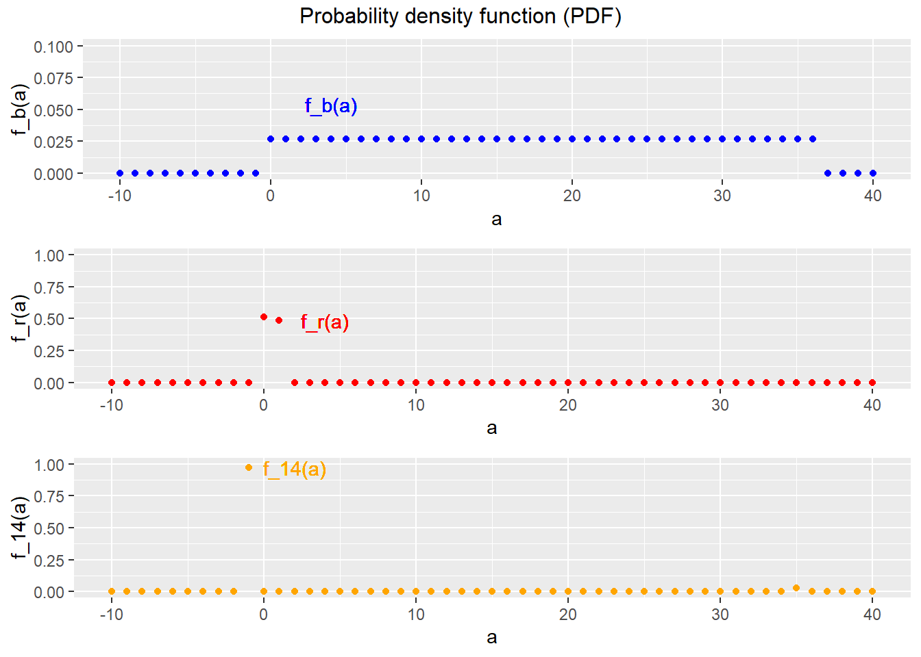
Figure 4.1: PDFs for the roulette example

You can also derive the probability distribution from the PDF. Again, we can make use of the idea of calculating event probabilities by adding up outcome probabilities. To calculate the probability that a random variable $x$ is in some set $A$, follow three steps:

List all values in $A$.
Use the PDF to calculate the probability of each value.
Add up the probabilities.

As in Section 3.3.3, we can summarize this procedure with a formula: \[\begin{align} \Pr(x \in A) &= \sum_{s \in A} \Pr(x = s) \\ &= \sum_{s \in S_x} f_x(s)I(s \in A) \end{align}\] and we can demonstrate the procedure by example.

Example 4.5 Some event probabilities in roulette

Since the outcome in roulette is discrete, we can calculate any event probability by adding up the probabilities of the event’s component outcomes.

The probability of the event $b \leq 1$ can be calculated: \[\begin{align} \Pr(b \leq 1) &= \sum_{s=0}^{36}f_b(s)I(s \leq 1) \\ &= \begin{aligned}[t] & \underbrace{f_b(0)}_{1/37} \underbrace{I(0 \leq 1)}_{1} + \underbrace{f_b(1)}_{1/37} \underbrace{I(1 \leq 1)}_{1} + \underbrace{f_b(2)}_{1/37} \underbrace{I(2 \leq 1)}_{0} \\ &+ \cdots + \underbrace{f_b(36)}_{1/37} \underbrace{I(36 \leq 1)}_{0} \\ \end{aligned} \\ &= 2/37 \end{align}\]

The probability of the event $b \in Even$ can be calculated: \[\begin{align} \Pr(b \in Even) &= \sum_{s=0}^{36}f_b(s)I(s \in Even) \\ &= \begin{aligned}[t] & \underbrace{f_b(0)}_{1/37} \underbrace{I(0 \in Even)}_{0} + \underbrace{f_b(1)}_{1/37} \underbrace{I(1 \in Even)}_{0} + \underbrace{f_b(2)}_{1/37} \underbrace{I(2 \in Even)}_{1} \\ &+ \cdots + \underbrace{f_b(36)}_{1/37} \underbrace{I(36 \in Even)}_{1} \\ \end{aligned} \\ &= 18/37 \end{align}\] Remember that zero is not counted as an even number in roulette, so it is not in the event $Even$.

The PDF of a discrete random variable therefore provides a compact but complete way of summarizing its probability distribution. It has several general properties:

It is always between zero and one: \[\begin{align} 0 \leq f_x(a) \leq 1 \end{align}\] since it is a probability.
It sums up to one over the support: \[\begin{align} \sum_{a \in S_x} f_x(a) = \Pr(x \in S_x) = 1 \end{align}\] since the support has probability one by definition.
It is strictly positive for all values in the support: \[\begin{align} a \in S_x \implies f_x(a) > 0 \end{align}\] since the support is the smallest set that has probability one.

You can confirm that examples above all satisfy these properties.

4.2.2 The CDF

Another way to describe the probability distribution of a random variable is with a function called its cumulative distribution function (CDF). The CDF is a little less intuitive than the PDF, but it has the advantage that it always has the same definition whether the random variable is discrete, continuous, or even some combination of the two.

The CDF of the random variable $x$ is the function $F_x:\mathbb{R} \rightarrow [0,1]$ defined by: \[\begin{align} F_x(a) = Pr(x \leq a) \end{align}\] where $a$ is any number. By convention, we typically use an upper-case $F$ to indicate a CDF, and we use the subscript to indicate what random variable we are talking about.

We can construct the CDF of a discrete random variable by just adding up the PDF. That is, for any value of $a$ we can calculate $F_x(a)$ by following three steps:

Find every value $s$ in the support of $x$ that is less than or equal to $a$.
Calculate the probability of each value using the PDF.
Add up the probabilities.

Expressed as a formula, this procedure is: \[\begin{align} F_x(a) &= \Pr(x \leq a) \\ &= \sum_{s \in S_x} f_x(s)I(s \leq a) \end{align}\] Again, the formula looks complicated but implementation is simple in practice.

Example 4.6 Deriving the CDF of $y_{14}$

We will derive the CDF $F_{14}(\cdot)$ of the random variable $y_{14}$ using the formula above and following this step-by-step procedure:

Write down the formula, substituting in the appropriate variable names: \[\begin{align} F_{14}(a) &= \Pr(y_{14} \leq a) \\ &= \sum_{s \in S_{14}} f_{14}(s)I(s \leq a) \end{align}\]
Find the support and substitute it into the formula. In this case, we earlier found that the support of $y_{14}$ is $S_{14} = \{-1, 35\}$ so: \[\begin{align} F_{14}(a) &= \sum_{s \in \{-1, 35\} } f_{14}(s)I(s \leq a) \end{align}\]
Expand out the summation: \[\begin{align} F_{14}(a) &= f_{14}(-1)I(-1 \leq a) + f_{14}(35)I(35 \leq a) \end{align}\] If you don’t know how to do this, review the material on summations in the Math Appendix.
Find the PDF and substitute it into the formula. In this case, we earlier found that $f_{14}(-1) = 36/37 \approx 0.973$ and $f_{14}(35) = 1/37 \approx 0.027$, so: \[\begin{align} F_{14}(a) &= 36/37 * I(-1 \leq a) + 1/37 * I(35 \leq a) \\ &\approx 0.973 * I(-1 \leq a) + 0.027 * I(1 \leq a) \\ \end{align}\]
Try out a few values for $a$. You can try as many values as you like until you get a feel for what this function looks like: \[\begin{align} F_{14}(-100) &\approx 0.973 * \underbrace{I (-1 \leq -100)}_{=0} + 0.027 * \underbrace{I(35 \leq -100)}_{=0} \\ &= 0 \\ F_{14}(-2) &\approx 0.973 * \underbrace{I (-1 \leq -2)}_{=0} + 0.027 * \underbrace{I(35 \leq -2)}_{=0} \\ &= 0 \\ F_{14}(-1) &\approx 0.973 * \underbrace{I (-1 \leq -1)}_{=1} + 0.027 * \underbrace{I(35 \leq -1)}_{=0} \\ &\approx 0.973 \\ F_{14}(0) &\approx 0.973 * \underbrace{I (-1 \leq 0)}_{=1} + 0.027 * \underbrace{I(35 \leq 0)}_{=0} \\ &\approx 0.973 \\ F_{14}(35) &\approx 0.973 * \underbrace{I (-1 \leq 35)}_{=1} + 0.027 * \underbrace{I(35 \leq 35)}_{=1} \\ &= 1 \\ F_{14}(100) &\approx 0.973 * \underbrace{I (-1 \leq 100)}_{=1} + 0.027 * \underbrace{I(35 \leq 100)}_{=1} \\ &= 1 \end{align}\]
Summarize your results in a clear and simple formula. Case notation is a good way to do this: \[\begin{align} F_{14}(a) &\approx \begin{cases} 0 & a < -1 \\ 0.973 & -1 \leq a < 35 \\ 1 & a \geq 35 \\ \end{cases} \end{align}\]

Figure 4.2 below shows this CDF. As you can see, it starts off at zero, jumps up at the values $-1$ and $35$ and then stays at one after that.

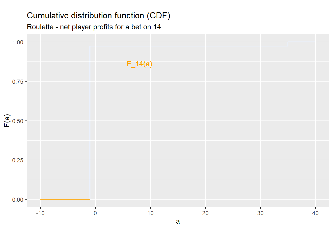
Figure 4.2: A CDF for the roulette example

I have given a specific formula and step-by-step instructions here, but once you have done a few of these calculations, you will probably be able to handle most cases without explicitly following each step. If you are stuck, come back to these instructions.

Example 4.7 More CDFs for roulette

We can follow the same procedure to derive CDFs for the other random variables:

The CDF of $b$ is: \[\begin{align} F_b(a) = \begin{cases} 0 & a < 0 \\ 1/37 & 0 \leq a < 1 \\ 2/37 & 1 \leq a < 2 \\ \vdots & \vdots \\ 36/37 & 35 \leq a < 36 \\ 1 & a \geq 36 \\ \end{cases} \end{align}\]
The CDF of $y_{14}$ is: \[\begin{align} F_{14}(a) = \begin{cases} 0 & a < -1 \\ 36/37 & -1 \leq a < 35 \\ 1 & a \geq 35 \\ \end{cases} \end{align}\]

If you plot a CDF you will notice it follows certain patterns.

Example 4.8 CDF properties

Figure 4.3 below graphs the CDFs from the previous example.

Notice that they show a few common properties:

The CDF runs from zero to one, and never leaves that range.
The CDF never goes down, it only goes up or stays the same.
The CDF has a distinctive “stair-step” shape, jumping up at each point in the support, and flat between those points,

In fact, the CDF of any discrete random variable has these properties.

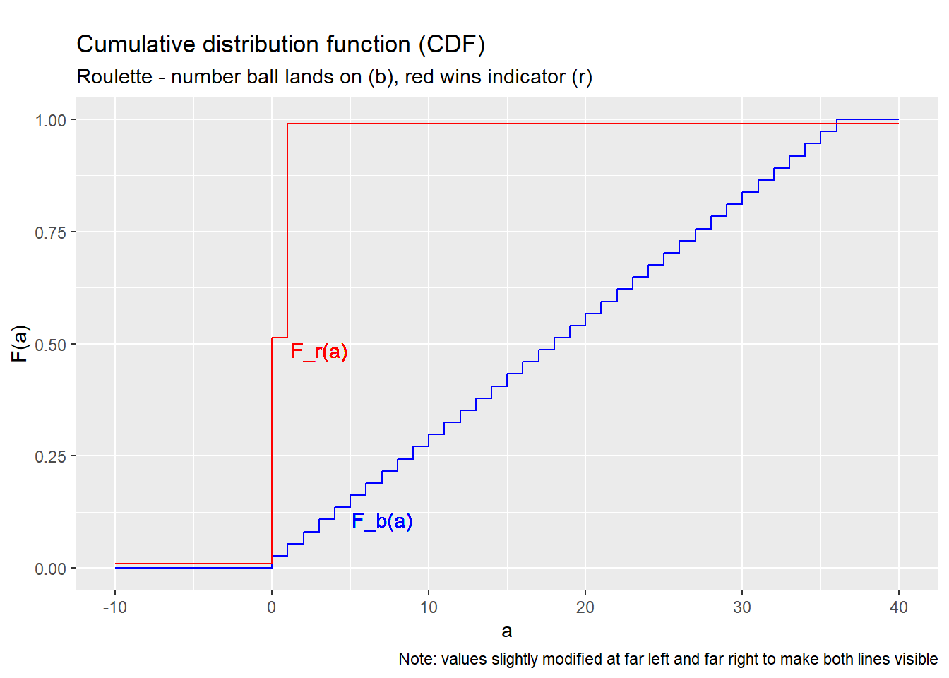
Figure 4.3: CDFs for the roulette example

All CDFs have the following properties:

The CDF is a probability, That is: \[\begin{align} 0 \leq F_x(a) \leq 1 \end{align}\] for any number $a$.
The CDF is non-decreasing. That is: \[\begin{align} F_x(a) \leq F_x(b) \end{align}\] for any two numbers $a$ and $b$ such that $a \leq b$.
The CDF runs from zero to one. That is, it is zero or close to zero for low values of $a$, and one or close to one for high values of $a$. We can use limits to give precise meaning to the broad terms “close”, “low”, and “high”: \[\begin{align} \lim_{a \rightarrow -\infty} F_x(a) = \Pr(x \leq -\infty) &= 0 \\ \lim_{a \rightarrow \infty} F_x(a) = \Pr(x \leq \infty) &= 1 \end{align}\] You can review the section on limits in the math appendix if you do not follow the notation.

In addition, all discrete random variables have the stair-step shape.

In addition to constructing the CDF from the PDF, we can also go the other way, and construct the PDF of a discrete random variable from its CDF. Each little jump in the CDF is a point in the support, and the size of the jump is exactly equal to the PDF.

In more formal mathematics, the formula for deriving the PDF of a discrete random variable from its CDF would be written: \[\begin{align} f_x(a) = F_x(a) - \lim_{\epsilon \rightarrow 0} F_x(a-|\epsilon|) \end{align}\] but we can just think of it as the size of the jump.

The table below summarizes the relationship between the probability distribution, the PDF, and the CDF. Since each of these functions provides a complete description of the associated random variable, we can choose to work with whichever is most convenient in a given application, and we can easily convert between them as needed.

Description	Probability distribution	PDF	CDF
Notation	$\Pr(A)$	$f_x(a)$	$F_x(a)$
Argument	An event (set) $A$	A number $a$	A number $a$
Value	$\Pr(x \in A)$	$\Pr(x = a)$	$\Pr(x \leq a)$
Fully describes distribution?	Yes	Yes	Yes

4.2.3 Interval probabilities

We can use the CDF to calculate the probability that $x$ lies in any interval. That is, let $L$ and $H$ be any two numbers such that $L < H$. Then the probability that $x$ is between $L$ and $H$ is given by: \[\begin{align} F_x(H) - F_x(L) &= \Pr(x \leq H) - \Pr(x \leq L) \\ &= \Pr((x \leq L) \cup (L < x \leq H)) - \Pr(x \leq L) \\ &= \Pr(x \leq L) + \Pr(L < x \leq H) - \Pr(x \leq L) \\ &= \Pr(L < x \leq H) \end{align}\] Notice that we have to be a little careful here to distinguish between the strict inequality $<$ and the weak inequality $\leq$, because it is always possible for $x$ to be exactly equal to $L$ or $H$. We can use the PDF as needed to adjust for those possibilities: \[\begin{align} \Pr(L < x \leq H) &= F_x(H) - F_x(L) \\ \Pr(L \leq x \leq H) &= \Pr(x = L) + \Pr(L < x \leq H) \\ &= f_x(a) + F_x(b) - F_x(a) \\ \Pr(L < x < H) &= \Pr(L < x \leq H) - \Pr(x = H) \\ &= F_x(H) - F_x(L) - f_x(H) \\ \Pr(L \leq x < H) &= \Pr(x = L) + \Pr(L < x \leq H) - \Pr(x = H) \\ &= f_x(L) + F_x(H) - F_x(L) - f_x(H) \end{align}\]

Example 4.9 Calculating interval probabilities

Consider the CDF for $b$ derived above. Then: \[\begin{align} \Pr(b \leq 36) &= F_b(36) \\ &= 1 \\ \Pr(1 < b \leq 36) &= F_b(36) - F_b(1) \\ &= 1 - 2/37 \\ &= 35/37 \end{align}\] Note that the placement of the $<$ and $\leq$ are important here.

What if we want $\Pr(1 \leq b \leq 36)$ instead? We can split that event into two disjoint events $(b = 1)$ and $(1 < b \leq 36)$ and apply the axioms of probability: \[\begin{align} \Pr(1 \leq b \leq 36) &= \Pr( (b = 1) \cup (1 < b \leq 36) ) \\ &= \Pr(b = 1) + \Pr(1 < b \leq 36) \\ &= f_b(1) + F_b(36) - F_b(1) \\ &= 1/37 + 1 - 2/37 \\ &= 36/37 \end{align}\] We can use similar methods to determine $\Pr(1 < b < 36)$ or $\Pr(1 \leq b < 36)$.

4.2.4 Range and mode

The range of a random variable is the interval from its lowest possible value to its highest possible value. It can be caclulated from the support: \[\begin{align} range(x) &= [\min(S_x), \max(S_x)] \end{align}\] or from the PDF or CDF.

Example 4.10 The range in roulette

The support of $y_{Red}$ is $\{-1,1\}$ so its range is $[-1,1]$.

The support of $y_{14}$ is $\{-1,35\}$ so its range is $[-1,35]$.

The support of $b$ is $\{0,1,2,\ldots,36\}$ so its range is $[0,36]$.

The mode of a discrete random variable is (loosely speaking) its most likely value. That is, it is the number $a$ that maximizes $\Pr(x=a)$. A random variable can have more than one mode, in which case the mode is a set of numbers.

Example 4.11 The mode in roulette

The mode of $r$ is $0$, since $f_{r}(0) = 0.514 > 0.486 = f_{r}(1)$.

The mode of $y_{Red}$ is $-1$, since $f_{Red}(-1) = 0.514 > 0.486 = f_{Red}(1)$.

The mode of $y_{14}$ is $-1$, since $f_{14}(-1) = 0.973 > 0.027 = f_{14}(35)$.

The mode of $b$ is the set $\{0,1,2,\ldots,36\}$ since each of those values has the same probability.

The mathematical language defining the mode is: \[\begin{align} mode(x) &= \textrm{arg }\max_{a \in S_x} f_x(a) \end{align}\]

4.3 The expected value

The expected value of a random variable $x$ is written $E(x)$. When $x$ is discrete, it is defined as: \[\begin{align} E(x) = \sum_{a \in S_x} a\Pr(x=a) = \sum_{a \in S_x} af_x(a) \end{align}\] The expected value is also called the mean, the population mean or the expectation of the random variable.

The formula for the expected value may look difficult if you are not used to the notation, but it is actually quite simple to calculate: just multiply each possible value by its probability, and then add it all up.

Example 4.12 Calculating the expected value of $y_{14}$

In previous examples, we found the support and PDF of $y_{14}$. We can find its expected value by following these steps:

Rewrite the formula with the correct variable names: \[\begin{align} E(y_{14}) &= \sum_{a \in S_{14}} a f_{14}(a) \end{align}\]
Find the support and substitute: \[\begin{align} E(y_{14}) &= \sum_{a \in \{-1,35\}} a f_{14}(a) \end{align}\]
Expand the summation: \[\begin{align} E(y_{14}) &= -1 * f_{14}(-1) + 35 * f_{14}(35) \end{align}\]
Find the PDF values and substitute: \[\begin{align} E(y_{14}) &= -1 * 36/37 + 35 * 1/37 \\ &= -1/37 \\ &\approx -0.027 \end{align}\]

The expected value of a random variable is an important concept, and has several closely related interpretations:

As a weighted average of its possible values, That is, it is like an average but instead of each value receiving equal weight it receives a weight equal to the probability that we will observe that value.
As a measure of central tendency, i.e., a typical or representative value for the random variable. Other measures of central tendency include the median and the mode.
As a prediction for the value of the random variable. That is, we want to predict/guess its value, and we want our guess to be as close as possible to the actual (not-yet-known) value. The median and mode are also used for prediction; the best prediction method depends on what you mean by “as close as possible”:
- The mode is is the most likely to be exactly correct (prediction error of zero).
- The median tends to produce the lowest absolute prediction error.
- The expected value tends to produce the lowest squared prediction error.

We can use whichever of these interpretations makes sense for a given application.

Example 4.13 Interpreting the expected value of $y_{14}$

As described earlier, we can think of the expected value as describing a typical or predicted value for the random variable. In this case, our result can be interpreted as a prediction of the house advantage: the player can expect to lose approximately 2.7 cents per dollar bet on 14, and the house can expect to gain approximately 2.7 cents per dollar bet on 14.

We can follow the same procedures to find and interpret the expected value of any discrete random variable.

Example 4.14 More expected values in roulette

The support of $b$ is $\{0,1,2\ldots,36\}$ and its PDF is the $f_b(\cdot)$ function we calculated earlier. So its expected value is: \[\begin{align} E(b) &= \sum_{a \in S_b} a f_b(a) \\ &= \sum_{a \in \{0,1,2\ldots,36\}} a f_b(a) \\ &= 0*\underbrace{f_b(0)}_{1/37} + 1*\underbrace{f_b(1)}_{1/37} + \cdots 36*\underbrace{f_b(36)}_{1/37} \\ &= \frac{1 + 2 + \cdots + 36}{37} \\ &= 18 \end{align}\]

The support of $r$ is $\{0,1\}$ and its PDF is the $f_r(\cdot)$ function we calculated earlier. So its expected value is: \[\begin{align} E(r) &= \sum_{a \in S_r} a f_r(a) \\ &= \sum_{a \in \{0,1\}} a f_r(a) \\ &= 0*\underbrace{f_r(0)}_{19/37} + 1*\underbrace{f_r(1)}_{18/37} \\ &= 18/37 \\ &\approx 0.486 \end{align}\]

4.4 Quantiles and their relatives

You have probably heard of the median, and you may have heard of percentiles. These are special cases of a group of numbers called the quantiles of a distribution.

4.4.1 Quantiles and percentiles

Let $q$ be any number strictly between zero and one. Then the $q$ quantile of a random variable $x$ is defined as: \[\begin{align} F_x^{-1}(q) &= \min\{a \in S_X: \Pr(x \leq a) \geq q\} \\ &= \min\{a \in S_x: F_x(a) \geq q\} \end{align}\] where $F_x(\cdot)$ is the CDF of $x$. The quantile function $F_x^{-1}(\cdot)$ is also called the inverse CDF of $x$. The $q$ quantile of a distribution is also called the $100q$ percentile; for example the 0.75 quantile of $x$ is also called the 75th percentile of $x$.

We can use the formula above to find quantiles from the CDF. The procedure is easier to follow if we do it graphically.

Example 4.15 Quantiles in roulette

Suppose we want to find the 0.25, 0.5, and 0.75 quantiles of the random variable $r$. We start by writing down the CDF: \[\begin{align} F_{r}(a) = \begin{cases} 0 & a < 0 \\ 19/37 \approx 0.514 & 0 \leq a < 1 \\ 1 & a \geq 1 \\ \end{cases} \end{align}\] Then we plot the CDF, as in Figure 4.4. To find any quantile $q$, we can apply the definition,or just need to find the value on the graph where $F_{r}(\cdot)$ crosses $q$.

For example, the 0.25 quantile (25th percentile) is defined as: \[\begin{align} F_{r}^{-1}(0.25) &= \min\{a \in S_x: F_{r}(a) \geq 0.25\} \\ &= \min \{0, 1\} \\ &= 0 \end{align}\] or we can draw the blue dashed line marked “0.25 quantile” and see that it hits the red line at $a = 0$. By the same method, we can find that the 0.5 quantile (50th percentile) is also zero.

Following this method again, we find the 0.75 quantile (75th percentile) by seeing that the red line crosses the blue dashed line marked “0.75 quantile” at $a = 1$, or we can apply the definition: \[\begin{align} F_{r}^{-1}(0.75) &= \min\{a \in S_x: F_{r}(a) \geq 0.75\} \\ &= \min \{1\} \\ &= 1 \end{align}\] Either method will work.

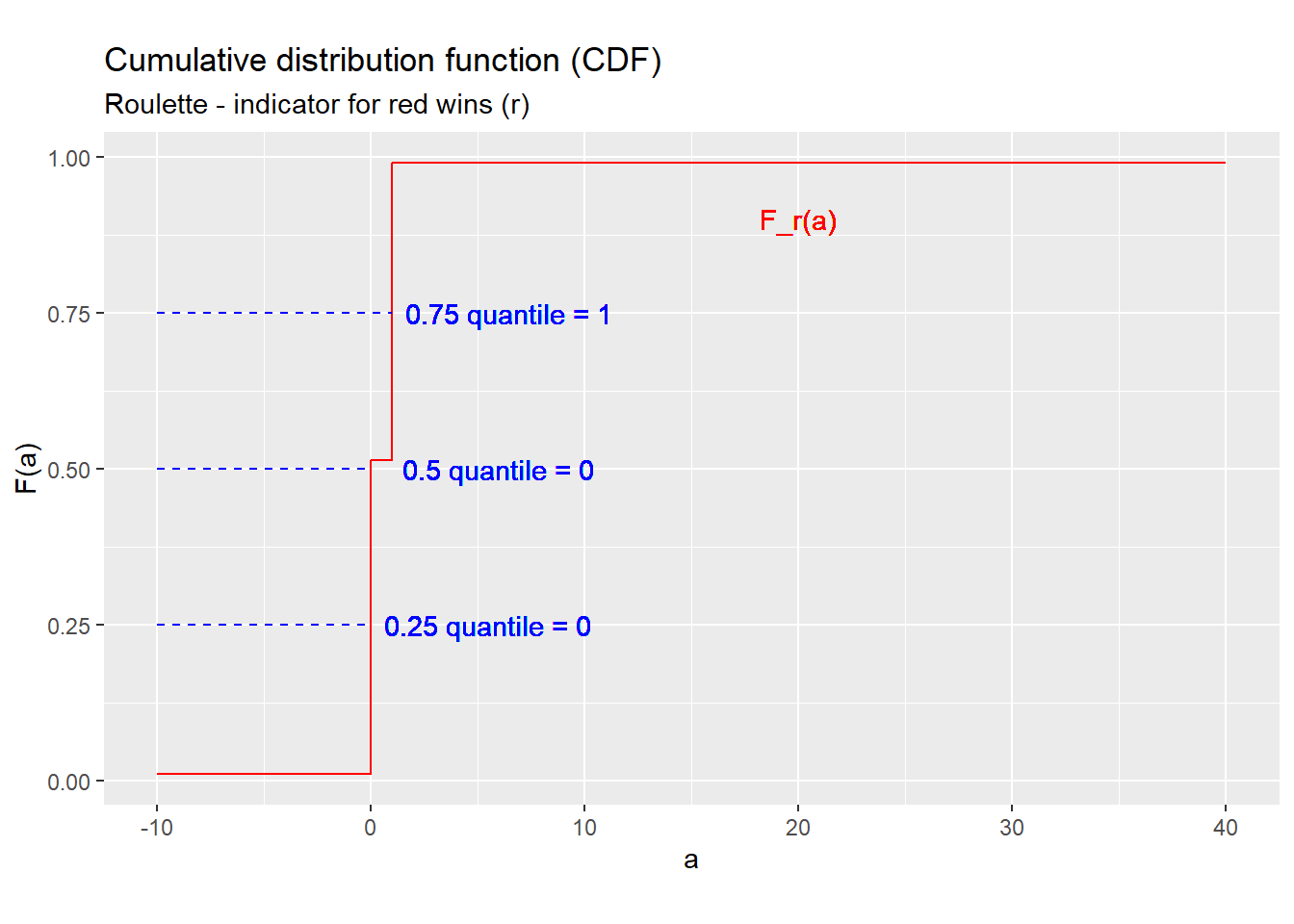
Figure 4.4: Deriving quantiles from the CDF

The formula for the quantile function may look intimidating, but it can be constructed by just “flipping” the axes of the CDF. This is why the quantile function is also called the inverse CDF.

Example 4.16 The whole quantile function

We can use the same ideas as in the previous example to show that $F_{r}^{-1}(q)$ is equal to $0$ for any $q$ between $0$ and $19/37$, and equal to $1$ for any $q$ between $19/37$ and $1$. But what is the value of $F^{-1}_{r}(19/37)$? To figure that out we will need to carefully apply the definition: \[\begin{align} F_{r}^{-1}(19/37) &= \min\{a \in S_x: F_{r}(a) \geq 19/37\} \\ &= \min \{-1,1\} \\ &= -1 \end{align}\] So the full quantile function can be written in case form as: \[\begin{align} F_{r}^{-1}(q) &= \begin{cases} 0 & 0 < q \leq 19/37 \\ 1 & 19/37 < q < 1 \\ \end{cases} \end{align}\] and we can plot it as in Figure 4.5 below. Notice that the quantile function looks just like the CDF, but with the horizontal and vertical axes flipped.

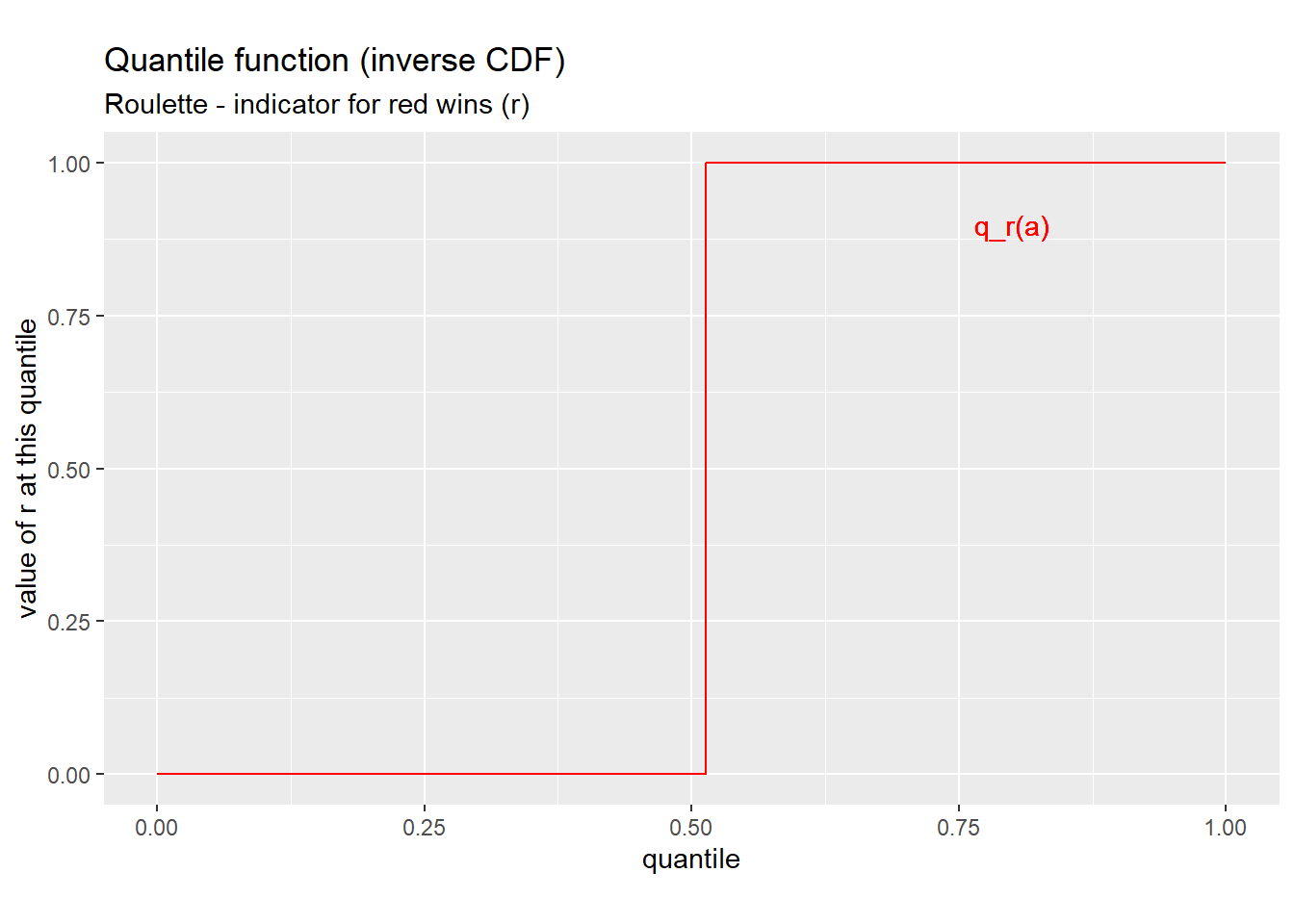
Figure 4.5: Quantile function for $r$

4.4.2 Median

The median of a random variable is its 0.5 quantile or 50th percentile.

Example 4.17 The median in roulette

The median of $r$ is just its 0.5 quantile or 50th percentile: \[\begin{align} median(r) = F_{r}^{-1}(0.5) = 0 \end{align}\]

Like the expected value, the median is often interpreted as a measure of central tendency for the random variable.

4.5 Functions of a random variable

Any function of a random variable is also a random variable. So for example, if $x$ is a random variable, so is $x^2$ or $\ln (x)$ or $\sqrt{x}$.

Example 4.18 The net profit from a bet on red ($y_{Red}$)

The player’s net profit from $1 bet on red $(y_{Red})$ was earlier defined directly from the underlying outcome $\omega$. \[\begin{align} y_{Red} &= \begin{cases} 1 & \textrm{ if } \omega \in RedWins \\ -1 & \textrm{ if } \omega \in RedWins^c \end{cases} \\ \end{align}\]

Alternatively, we can define it in terms of the random variable $b$, or of the random variable $r$: \[\begin{align} y_{Red} &= 2I(b \in RedWins) - 1 \\ y_{Red} &= 2r -1 \end{align}\] where $I(\cdot)$ is the indicator function.

When $y$ is a function of $x$, we can derive the probability distribution of $y$ directly from the probability distribution of $x$, using the same method we used in Section 4.1.1. We can also use a similar formula: \[\begin{align} E( h(x) ) &= \sum_{s \in S_x} h(s) f_x(s) \end{align}\] to calculate the expected value of $y = h(x)$ from the PDF of $x$.

Example 4.19 The expected value of $y_{14}^2$

Suppose we are interested in the expected value of $y_{14}^2$ - it’s not obvious why we would be, but we will be.

Applying the formula above we get: \[\begin{align} E(y_{14}^2) &= \sum_{s \in S_{14}} s^2 f_{14}(s) \\ &= \sum_{s \in \{-1, 35\}} s^2 f_{14}(s) \\ &= (-1)^2 f_{14}(-1) + 35^2 f_{14}(35) \\ &= 1 * 36/37 + 1225 * 1/37 \\ &\approx 34.1 \end{align}\] This result will turn out to be useful later.

We say that $y$ is a linear function of $x$ when we can write it in the form: \[\begin{align} y &= a + bx \end{align}\] for some constants $a$ and $b$. When $y$ is a function of $x$ but cannot be written in this form, we say that it is a nonlinear function of $x$.

Example 4.20 Linear and nonlinear functions in roulette

The player’s net profit from a bet on red is a linear function of the random variable $r$: \[\begin{align} y_{Red} = 2r -1 \end{align}\] and it is a nonlinear function of the random variable $b$: \[\begin{align} y_{Red} = 2I(b \in RedWins) - 1 \end{align}\]

Linear functions are particularly convenient to work with. In particular, we can prove that the expected value of any linear function of any random variable $x$ is: \[\begin{align} E(a + bx) &= a + b E(x) \end{align}\] That is, we do not need to know the entire distribution of $x$ to calculate $E(y)$; we only need to know the expected value $E(x)$.

Example 4.21 The expected value of $y_{Red}$

Earlier, we showed that $y_{Red}$ can be defined as a linear function of $r$: \[\begin{align} y_{Red} = 2r -1 \end{align}\] so its expected value can be derived: \[\begin{align} E(y_{Red}) &= E(2r - 1) \\ &= 2 \underbrace{E(r)}_{18/37} - 1 \\ &= -1/37 \\ &\approx -0.027 \end{align}\] We can interpret this result as saying that the house advantage for bets on red is 2.7 cents per dollar bet. Note that this is the same house advantage as we earlier derived for a bet on 14.

Unfortunately, this handy property applies only to linear functions.

Never take the expected value inside a nonlinear function

If $h(\cdot)$ is a linear function, than $E(h(x)) = h(E(x))$.

But if $h(\cdot)$ is a nonlinear function, than $E(h(x)) \neq h(E(x))$.

Students frequently make this mistake, so try to avoid it.

We can see this with an example.

Example 4.22 The expected value of a nonlinear function in roulette

We can define $y_{Red}$ as a nonlinear function of $b$: \[\begin{align} y_{Red} = 2 I(b \in RedWins) - 1 \end{align}\] Can we take the expected value “inside” of this function? That is, does $E(y_{Red}) = 2 I(E(b) \in RedWins) - 1$?

The answer to this question is “No”. We already showed that $E(y_{Red}) \approx -0.027$. We also showed earlier that $E(b) = 18$, so we can find: \[\begin{align} 2 I(E(b) \in RedWins) - 1 &= 2 I(18 \in RedWins) - 1 \\ &= 2*1 - 1 \\ &= 1 \end{align}\] Since $-0.027 \neq 1$, it is clear that $E(y_{Red})$ is not equal to $2 I(E(b) \in RedWins) - 1$.

More generally, there is no formula that would allow you to calculate the expected value $E(y_{Red})$ using only the expected value $E(b)$. You need the whole distribution of $b$ to calculate $E(y_{Red})$.

The expected value is a sum!

The result that $E(a + bx) = a + b E(x)$ is one that we will use repeatedly. While proving it is not something I would ask you to do, working through the proof is useful in understanding why it works, and why the result only applies to linear functions of $x$.

The key to all of this is that the expected value is a sum. Consider the formula for the expected value above: \[\begin{align} E( h(x) ) &= \sum_{s \in S_x} h(s) f_x(s) \end{align}\] When $y = h(x)$ is a linear function of $x$, this reduces to: \[\begin{align} E(y) &= E( a + bx ) \\ &= \sum_{s \in S_x} (a + bs) f_x(s) \end{align}\] At this point, remember three rules of arithmetic you learned in grade school. The first rule is the distributive property of multiplication, which says that $a*(b+c) = a*b + a*c$. This allows us to rearrange: \[\begin{align} E(y) &= \sum_{s \in S_x} (a + bs) f_x(s) \\ &= \sum_{s \in S_x} a f_x(s) + bs f_x(s) \end{align}\] The other two rules are that you can rearrange a sum in any order you like (this is called the commutative property of addition: $a + b = b + a$), and that you can group sums in any way you like (the associative property of addition: $(a + b) + c = a + (b + c)$). This allows us to rearrange the summations like this: \[\begin{align} E(y) &= \sum_{s \in S_x} a f_x(s) + bs f_x(s) \\ &= \sum_{s \in S_x} a f_x(s) + \sum_{s \in S_x} bs f_x(s) \end{align}\] Then we apply the commutative property again: \[\begin{align} E(y) &=\sum_{s \in S_x} a f_x(s) + \sum_{s \in S_x} bs f_x(s) \\ &= a \underbrace{\sum_{s \in S_x} f_x(s)}_{= 1} + b \underbrace{\sum_{s \in S_x} s f_x(s)}_{=E(x)} \\ &= a + bE(x) \end{align}\] to get our result.

4.6 Variance and standard deviation

In addition to measures of central tendency such as the expected value and median, we are also interested in measures of “spread” or variability. We have already seen one - the range - but there are others, including the variance and the standard deviation.

4.6.1 Variance

The variance of a random variable $x$ is defined as: \[\begin{align} \sigma_x^2 = var(x) = E((x-E(x))^2) \end{align}\] where $\sigma$ is the lower-case Greek letter sigma.

Variance can be thought of as a measure of how much $x$ tends to deviate from its central tendency $E(x)$.

Example 4.23 Calculating variance from the PDF

We can calculate the variance of $r$ directly from its PDF: \[\begin{align} var(r) &= E( (r - E(r))^2 ) \\ &= \sum_{s \in S_r} (s - E(r) )^2 f_r(s) \\ &= \sum_{s \in \{0, 1\}} (s - E(r) )^2 f_r(s) \\ &= (0 - E(r) )^2 f_r(0) + (1 - E(r) )^2 f_r(1) \\ &\approx (0 - 0.486 )^2 * 0.514 + (1 - 0.486 )^2 * 0.486 \\ &\approx 0.25 \end{align}\] Note that we used the formula for the expected value of a function of a random variable, then substituted, expanded the sum, and substituted again to get the result.

The key to understanding the variance is that it is the expected value of a square $(x-E(x))^2$, and the expected value is just a (weighted) sum. This has several implications:

The variance is always positive (or more precisely, non-negative): \[\begin{align} var(x) \geq 0 \end{align}\] The intuition for this result is straightforward: the square of any number is always positive, and the expected value is just a sum. The variance is therefore a sum of several positive numbers, so it is also a positive number.
The variance can also be written in the form: \[\begin{align} var(x) = E(x^2) - E(x)^2 \end{align}\] The derivation of this is as follows: \[\begin{align} var(x) &= E((x-E(x))^2) \\ &= E( ( x-E(x) ) * (x - E(x) )) \\ &= E( x^2 - 2xE(x) + E(x)^2) \\ &= E(x^2) - 2E(x)E(x) + E(x)^2 \\ &= E(x^2) - E(x)^2 \end{align}\] This formula is often an easier way of calculating the variance.

Example 4.24 Calculating variance using the alternate formula

We can use the alternative formula to calculate $var(y_{14})$.

Calculate $E(y_{14})$ from the PDF of $y_{14}$. We found this earlier: \[\begin{align} E(y_{14}) &\approx -0.027 \end{align}\]
Calculate $E(y_{14}^2)$ from the PDF of $y_{14}$. We also found this earlier: \[\begin{align} E(y_{14}^2) &\approx 34.1 \end{align}\]
Put these two results into the formula: \[\begin{align} var(y_{14}) &= E(y_{14}^2) - E(y_{14})^2 \\ &\approx 34.1 - (-0.027)^2 \\ &\approx 34.1 \end{align}\]

This is the same result you would get if you calculated $var(y_{14})$ directly from the PDF, but you may find it easier to calculate.

We can also find the variance of any linear function of a random variable. For any constants $a$ and $b$: \[\begin{align} var(a + bx) = b^2 var(x) \end{align}\] This can be derived as follows: \[\begin{align} var(a+bx) &= E( ( (a+bx) - E(a+bx))^2) \\ &= E( ( a+bx - a-bE(x))^2) \\ &= E( (b(x - E(x)))^2) \\ &= E( b^2(x - E(x))^2) \\ &= b^2 E( (x - E(x))^2) \\ &= b^2 var(x) \end{align}\]

Example 4.25 Calculating the variance of a linear function

We earlier found that $var(r) \approx 0.25$ and that $y_{Red} = 2r - 1$. So we can use our formula for the variance of a linear function to find the variance of $y_{Red}$ : \[\begin{align} var(y_{Red}) &= var( 2r - 1) \\ &= 2^2 var(r) \\ &\approx 4*0.25 \\ &\approx 1.0 \end{align}\] This is much easier than doing the calculation directly from the PDF.

The variance has a natural interpretation as a measure of how much the random variable tends to vary. Low variance means you get similar results each time, high variance means that results vary a lot.

Example 4.26 Interpreting the variance of $y_{Red}$ and $y_{14}$

We earlier found that a bet on red and a bet on 14 have the same expected value: \[\begin{align} E(y_{red}) &\approx -0.027 \\ E(y_{14}) &\approx -0.027 \end{align}\] However, a bet on red has a much lower variance: \[\begin{align} var(y_{red}) &\approx 1.0 \\ var(y_{14}) &\approx 34.1 \end{align}\] What this means in the context of betting is that all players will tend to lose money on average with both bets (low and negative expected value) but most players who bet on red will tend to have similar results (most players lose their money slowly) while players who bet on 14 will tend to have more variable results (a few players will have a big win or two, while most players lose their money quickly).

4.6.2 Standard deviation

The standard deviation of a random variable is defined as the (positive) square root of its variance: \[\begin{align} \sigma_x = sd(x) = \sqrt{var(x)} \end{align}\] The standard deviation is just another way of describing the variability of $x$.

In some sense, the variance and standard deviation are interchangeable since they are so closely related. The standard deviation has the advantage that it is expressed in the same units as the underlying random variable, while the variance is expressed in the square of those units. This makes the standard deviation somewhat easier to interpret.

Example 4.27 Standard deviation in roulette

The standard deviation of $r$ is: \[\begin{align} sd(r) = \sqrt{var(r)} \approx \sqrt{0.25} \approx 0.5 \end{align}\]

The standard deviation of $y_{Red}$ is: \[\begin{align} sd(y_{Red}) = \sqrt{var(y_{Red})} \approx \sqrt{1.0} \approx 1.0 \end{align}\] The standard deviation of $y_{14}$ is: \[\begin{align} sd(y_{14}) = \sqrt{var(y_{14})} \approx \sqrt{34.1} \approx 5.8 \end{align}\]

The standard deviation has analogous properties to the variance:

It is always non-negative: \[\begin{align} sd(x) \geq 0 \end{align}\]
For any constants $a$ and $b$: \[\begin{align} sd(a + bx) = |b| \, sd(x) \end{align}\] where $|b|$ is the absolute value of $b$.

These properties follow directly from the corresponding properties of the variance.

Example 4.28 Calculating the standard deviation of a linear function

We earlier found that $sd(r) \approx 0.5$ and that $y_{Red} = 2r - 1$. So we can use our formula for the standard deviation of a linear function to find the standard deviation of $y_{Red}$ : \[\begin{align} sd(y_{Red}) &= sd( 2r - 1) \\ &= 2 sd(r) \\ &\approx 2*0.5 \\ &\approx 1.0 \end{align}\] As expected, this is the same answer we found in the previous example.

4.6.3 Standardization

In some cases, it is useful to standardize a random variable. This means constructing a new random variable of the form: \[\begin{align} z &= \frac{x - E(x)}{sd(x)} \end{align}\] where $x$ is the original random variable and $z$ is the standardized version of $x$. That is, we subtract the expected value, and divide by the standard deviation.

Standardization is an example of a change in units, just like converting miles to kilometers, or grams to kilograms. Like most changes in units, it is a linear transformation. That is, we can rewrite $z$ as a linear function of $x$: \[\begin{align} z &= \frac{-E(x)}{sd(x)} + \frac{1}{sd(x)} * x \end{align}\] We can also use our rules for linear functions of a random variable to get: \[\begin{align} E(z) &= \frac{-E(x)}{sd(x)} + \frac{1}{sd(x)} * E(x) \\ &= 0 \\ var(z) &= \left(\frac{1}{sd(x)}\right)^2 * var(x) \\ &= 1 \end{align}\] That is, standardization rescales the variable to have a mean of zero and a variance or standard deviation of one.

Standardization is commonly used in fields like psychology or educational testing when a variable has no natural unit of measurement.

Example 4.29 A standardized test score

Suppose that the midterm exam in this course is graded on a scale from 0 to 60 points, with a mean score of $E(x) = 40$ and a standard deviation of $sd(x) = 10$. For any individual student’s score $x$, the standardized score is: \[\begin{align} z = \frac{x-40}{10} \end{align}\] or (equivalently): \[\begin{align} z = 0.1 x - 4 \end{align}\] Applying our results on linear functions of a random variable: \[\begin{align} E(z) &= 0.1 E(x) - 4 \\ &= 0.1 \times 40 - 4 \\ &= 0 \\ sd(z) &= 0.1 sd(x) \\ &= 0.1 \times 10 \\ &= 1 \end{align}\] For example, a student with a test score of 45 would have a standardized score of $z = (45-40)/10 = 0.5$ meaning their original score was 0.5 standard deviations above the average score. Another student with a test score of 30 would have a standardized score of $z = (30-40)/10 = -1$, meaning their original score was one standard deviation below the average score.

4.7 Standard discrete distributions

In principle, there are an infinite number of possible probability distributions. However, some probability distributions are common enough in applications that we have given them names. This provides a quick way to describe a particular distribution without writing out its full PDF, using the notation: \[\begin{align} RandomVariable \sim DistributionName(Parameters) \end{align}\] where $RandomVariable$ is the name of the random variable whose distribution is being described, the $\sim$ character can be read as “has the following probability distribution”, $DistributionName$ is the name of the probability distribution, and $Parameters$ is a list of arguments (usually numbers) called parameters that provide additional information about the probability distribution.

Using a standard distribution also allows us to establish the properties of a commonly-used distribution once, and use those results every time we use that distribution. In this section we will describe three standard distributions - the Bernoulli, the binomial, and the discrete uniform - and their properties.

4.7.1 Bernoulli

The Bernoulli probability distribution is usually written: \[\begin{align} x \sim Bernoulli(p) \end{align}\] It has discrete support $S_x = \{0,1\}$ and PDF: \[\begin{align} f_x(a) &= \begin{cases} (1-p) & \textrm{if $a = 0$} \\ p & \textrm{if $a = 1$} \\ 0 & \textrm{otherwise}\\ \end{cases} \end{align}\] Note that the “Bernoulli distribution” isn’t really a (single) probability distribution. Instead it is what we call a parametric family of distributions. That is, the $Bernoulli(p)$ is a different distribution with a different PDF for each value of the parameter $p$.

We typically use Bernoulli random variables to model the probability of some random event $A$. If we define $x$ as the indicator variable $x=I(A)$, then $x \sim Bernoulli(p)$ where $p=\Pr(A)$.

Example 4.30 The Bernoulli distribution in roulette

The variable $r = I(\omega \in RedWins)$ has the $Bernoulli(18/37)$ distribution.

The mean of a $Bernoulli(p)$ random variable is: \[\begin{align} E(x) &= (1-p)*0 + p*1 \\ &= p \end{align}\] and its variance is: \[\begin{align} var(x) &= E(x^2) - E(x)^2 \\ &= (0^2*(1-p) + 1^2 p) - (p)^2 \\ &= p - p^2 \end{align}\] If you recognize that a particular random variable has a Bernoulli distribution, you can use these two results to save yourself the trouble of doing the calculations by hand.

4.7.2 Binomial

The binomial probability distribution is usually written: \[\begin{align} x \sim Binomial(n,p) \end{align}\] It has discrete support $S_x = \{0,1,2,\ldots,n\}$ and its PDF is: \[\begin{align} f_x(a) = \begin{cases} \frac{n!}{a!(n-a)!} p^a(1-p)^{n-a} & \textrm{if $a \in S_x$} \\ 0 & \textrm{otherwise} \\ \end{cases} \end{align}\] You do not need to memorize or even understand this formula. The Excel function BINOMDIST() can be used to calculate the PDF or CDF of the binomial distribution, and the function BINOM.INV() can be used to calculate its quantiles.

The binomial distribution is typically used to model frequencies or counts, because it is the distribution of how many times a probability-$p$ event happens in $n$ independent attempts.

Example 4.31 The binomial distribution in roulette

Suppose we play 50 (independent) games of roulette, and bet on red in every game. Since the outcome of a single bet on red is $r \sim Bernoulli(18/37)$, the number of times we win is: \[\begin{align} WIN50 \sim Binomial(50,18/37) \end{align}\] We can use the Excel formula =BINOM.DIST(25,50,18/37,FALSE) to calculate the probability of winning exactly 25 times: \[\begin{align} \Pr(WIN50 = 25) \approx 0.11 \end{align}\] we can use the Excel formula = BINOM.DIST(25,50,18/37,TRUE) to calculate the probability of winning 25 times or less: \[\begin{align} \Pr(WIN50 \leq 25) \approx 0.63 \end{align}\] and we can use the Excel formula = 1 - BINOM.DIST(25,50,18/37,TRUE) to calculate the probability of winning more than 25 times: \[\begin{align} \Pr(WIN50 > 25) = 1 - \Pr(WIN50 \leq 25) \approx 0.37 \end{align}\] So we have a 37% chance of making money (winning more often than losing), an 11% chance of breaking even, and a 52% chance of losing money. Notice that the chance of losing money over the course of 50 games (52%) is greater than the chance of losing money in a single game (51.4%). If you play enough games, the chance of losing money becomes very close to 100%.

The mean and variance of a binomial random variable are: \[\begin{align} E(x) &= np \\ var(x) &= np(1-p) \end{align}\] Again, if you recognize a random variable as having a binomial distribution you can use these results to save yourself the trouble of doing the calculations by hand.

Example 4.32 The binomial distribution in roulette, part 2

The number of wins in 50 bets on red has expected value: \[\begin{align} E(WIN50) = np = 50 * 18/37 \approx 24.3 \end{align}\] variance: \[\begin{align} var(WIN50) = np(1-p) = 50 * 18/37 * 19/37 \approx 12.5 \end{align}\] and standard deviation: \[\begin{align} sd(WIN50) = \sqrt{var(WIN50)} \approx \sqrt{12.5} \approx 3.5 \end{align}\]

The formula for the binomial PDF looks strange, but it can actually be derived from a fairly simple and common situation. Let our outcome $\omega = (b_1,b_2,\ldots,b_n)$ be a sequence of $n$ independent random variables from the $Bernoulli(p)$ distribution and let: \[\begin{align} x = \sum_{i=1}^n b_i \end{align}\] count up the number of times that $b_i$ is equal to one (i.e., the event modeled by $b_i$ happened). Then it is possible to derive the PDF for $y$, and that is the PDF we call $Binomial(n,p)$. The derivation is not easy, but the intuition is simple:

List every outcome in the event $x=a$. By a standard result about permutations (you would have learned this in grade 10 or so, don’t worry if you don’t remember it), there are exactly $\frac{n!}{a!(n-a)!}$ such outcomes.
By independence, each of these outcomes has probability $p^a(1-p)^{n-a}$.
We can calculate the probability of the event $x=a$ by adding up these probabilities.

Therefore the probability of the event $x=a$ is $\frac{n!}{a!(n-a)!}p^a(1-p)^{n-a}$.

4.7.3 Discrete uniform

The discrete uniform distribution: \[\begin{align} x \sim DiscreteUniform(S_x) \end{align}\] puts equal probability on every value in some discrete set $S_x$. Therefore, its support is $S_x$ and its PDF is: \[\begin{align} f_x(a) = \begin{cases} 1/|S_x| & a \in S_x \\ 0 & a \notin S_x \\ \end{cases} \end{align}\] Discrete uniform distributions appear in gambling and similar applications.

Example 4.33 The discrete uniform distribution in roulette

In our roulette example, the random variable $b$ has the $DiscreteUniform(\{0,1,\ldots,36\})$ distribution.

Chapter review

Random variables are simply numerical random outcomes. Economics is a primarily quantitative field, in the sense that most outcomes we study are numbers. This quantification helps us be more precise in our analysis and predictions, though it can miss important details that might be captured using qualitative or verbal methods like case studies and interviews.

In this chapter, we have learned various ways of describing the probability distribution of a simple random variable - a single random variable that takes on values in a finite set. We have also learned some standard probability distributions that are used to describe simple random variables.

Later in the course, we will deal with more complex random variables including random variables that take on values in a continuous set, as well as pairs or groups of related random variables. We will then apply the concept of a random variable to statistics calculated from data.

Practice problems

Answers can be found in the appendix.

The questions below continue our craps example. To review that example, we have an outcome $(r,w)$ where $r$ and $w$ are the numbers rolled on a pair of fair six-sided dice.

Let the random variable $t$ be the total showing on the pair of dice, and let the random variable $y = I(t=11)$ be an indicator for whether a bet on “Yo” wins.

GOAL #1: Define a random variable in terms of a random outcome

Define $t$ in terms of the underlying outcome $(r,w)$.
Define $y$ in terms of the underlying outcome $(r,w)$.

GOAL #2: Determine the support and range of a random variable

Find the support of the following random variables:
1. Find the support $S_r$ of the random variable $r$.
2. Find the support $S_t$ of the random variable $t$.
3. Find the support $S_y$ of the random variable $y$.
Find the range of each of the following random variables:
1. Find the range of $r$.
2. Find the range of $t$.
3. Find the range of $y$.

GOAL #3: Calculate and interpret the PDF of a discrete random variable

Find the following PDFs:
1. Find the PDF $f_r$ for the random variable $r$.
2. Find the PDF $f_t$ for the random variable $t$.
3. Find the PDF $f_y$ for the random variable $y$.

GOAL #4: Calculate and interpret the CDF of a discrete random variable

Using the PDFs you found earlier, find the following CDFs:
1. Find the CDF $F_r$ for the random variable $r$.
2. Find the CDF $F_y$ for the random variable $y$.

GOAL #5: Calculate interval probabilities from the CDF

Suppose that the discrete random variable $x$ has CDF $F_x$ where $F_x(0) = 0.3$, $F_x(5) = 0.8$, $f_x(0) = 0.1$, and $f_x(5) = 0.1$. Find the following interval probabilities:
1. Find $\Pr(x \leq 5)$.
2. Find $\Pr(x < 5)$.
3. Find $\Pr(x > 5)$.
4. Find $\Pr(x \geq 5)$.
5. Find $\Pr(0 < x \leq 5)$.
6. Find $\Pr(0 \leq x \leq 5)$.
7. Find $\Pr(0 < x < 5)$.
8. Find $\Pr(0 \leq x < 5)$.

GOAL #6: Calculate the expected value of a discrete random variable from its PDF

Using the PDFs you found earlier, find the following expected values:
1. Find the expected value $E(r)$.
2. Find the expected value $E(r^2)$.

GOAL #7: Calculate a quantile from the CDF

Using the CDFs you found earlier, find the following quantiles:
1. Find the median $Med(r)$.
2. Find the 0.25 quantile $F_r^{-1}(0.25)$.
3. Find the 75th percentile of $r$.

GOAL #8: Calculate the variance of a discrete random variable from its PDF

Let $d = (y - E(y))^2$.
1. Find the PDF $f_d$ of $d$.
2. Use this PDF to find $E(d)$
3. Use these results to find the variance $var(y)$.

GOAL #9: Calculate the variance from expected values

In question (8) above, you calculated $E(r)$ and $E(r^2)$ from the PDF. Use these results to find $var(r)$.

GOAL #10: Calculate the standard deviation from the variance

Find the following standard deviations:
1. Find $sd(y)$. You can use your result from question (10) above.
2. Find $sd(r)$. You can use your result from question (11) above.

GOAL #11: Calculate the expected value for a linear function of a random variable
GOAL #12: Calculate variance and standard deviation for a linear function of a random variable

The “Yo” bet pays out at 15:1, meaning you win $15 for each dollar bet. Suppose you bet $10 on Yo. Your net winnings in that case will be $W = 160*y - 10$.
1. Using earlier results, find $E(W)$.
2. Using earlier results, find $var(W)$.
3. The event $W > 0$ (your net winnings are positive) is identical to the event $y = 1$. Using earlier results, find $\Pr(W > 0)$.
Suppose you bet $1 on Yo in ten independent rolls. Your net winnings in that case will be $W_{10} = 16*Y_{10} - 10$.
1. Using earlier results, find $E(W_{10})$.
2. Using earlier results, find $var(W_{10})$.
3. The event $W_{10} > 0$ (your net winnings are positive) is identical to the event $Y_{10} > 10/16$. Using earlier results, find $\Pr(W_{10} > 0)$.

GOAL #13: Standardize a random variable

Let $z$ be the standardized form of the random variable $y$.
1. What is the formula defining $z$? Use actual numbers for $E(y)$ and $sd(y)$.
2. Find the support of $z$.
3. Find the PDF of $z$.

GOAL #14: Use standard standard discrete probability distributions

The random variable $y$ can be described using a standard distribution.
1. What standard distribution describes $y$?
2. Use standard results for this distribution to find $E(y)$
3. Use standard results for this distribution to find $var(y)$
Let $Y_{10}$ be the number of times in 10 dice rolls that a bet on “Yo” wins.
1. What standard distribution describes $Y_{10}$?
2. Use existing results for this distribution to find $E(Y_{10})$.
3. Use existing results for this distribution to find $var(Y_{10})$.
4. Use Excel to calculate $\Pr(Y_{10} = 0)$.
5. Use Excel to calculate $\Pr(Y_{10} \leq 10/16)$.
6. Use Excel to calculate $\Pr(Y_{10} > 10/16)$.

Technically, it is the smallest closed set, but let’s ignore that.↩︎

Description	Probability distribution	PDF	CDF
Notation	\(\Pr(A)\)	\(f_x(a)\)	\(F_x(a)\)
Argument	An event (set) \(A\)	A number \(a\)	A number \(a\)
Value	\(\Pr(x \in A)\)	\(\Pr(x = a)\)	\(\Pr(x \leq a)\)
Fully describes distribution?	Yes	Yes	Yes