Chapter 4 The Normal Distribution

Standard Deviation is a very useful number. In the case of normal distributions, which are ubiquitous in our lives, standard deviation can help us evaluate a measurement.

4.1 Why is the Normal Distribution so important?

The normal distribution, aka the bell curve, is everywhere. Many human physical and mental measurements form a rough bell curve if you gather a big enough sample.

Why is that?

Consider these seemingly unrelated questions: If you are to bet money on a fair dice roll, which number would you bet on?

If you are to bet money on the sum of two fair dice rolls, which number would you bet on?

The answer to the first question is any number between 1 to 6. But the answer to the second question is much more specific–you should bet on 7, because the two dice rolls would generate more combinations that add up to 7 than any other sums, as illustrated in the following picture:

We can also use R to roll the dice for us much more efficiently.

Roll a Die:

die=c(1,2,3,4,5,6)
sample(die,1)

## [1] 3

Now roll a die 10,000 times and plot the frequencies of each number:

roll1<-NULL
for (i in 1:10000) {
  a=sample(die,1)
  roll1=c(roll1,a)
}
hist(roll1)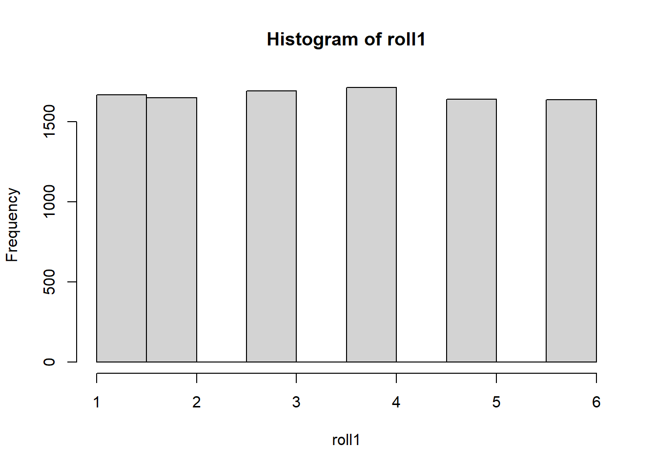

The histogram shows that all numbers from 1 to 6 have roughly the same chance of being rolled.

Roll two dice 10,000 times and plot the frequency of the sums

roll2=NULL
for (i in 1:10000){
  a=sample(die,1)+sample(die,1)
  roll2=c(roll2,a)
}
hist(roll2, main="sum of 2 rolls")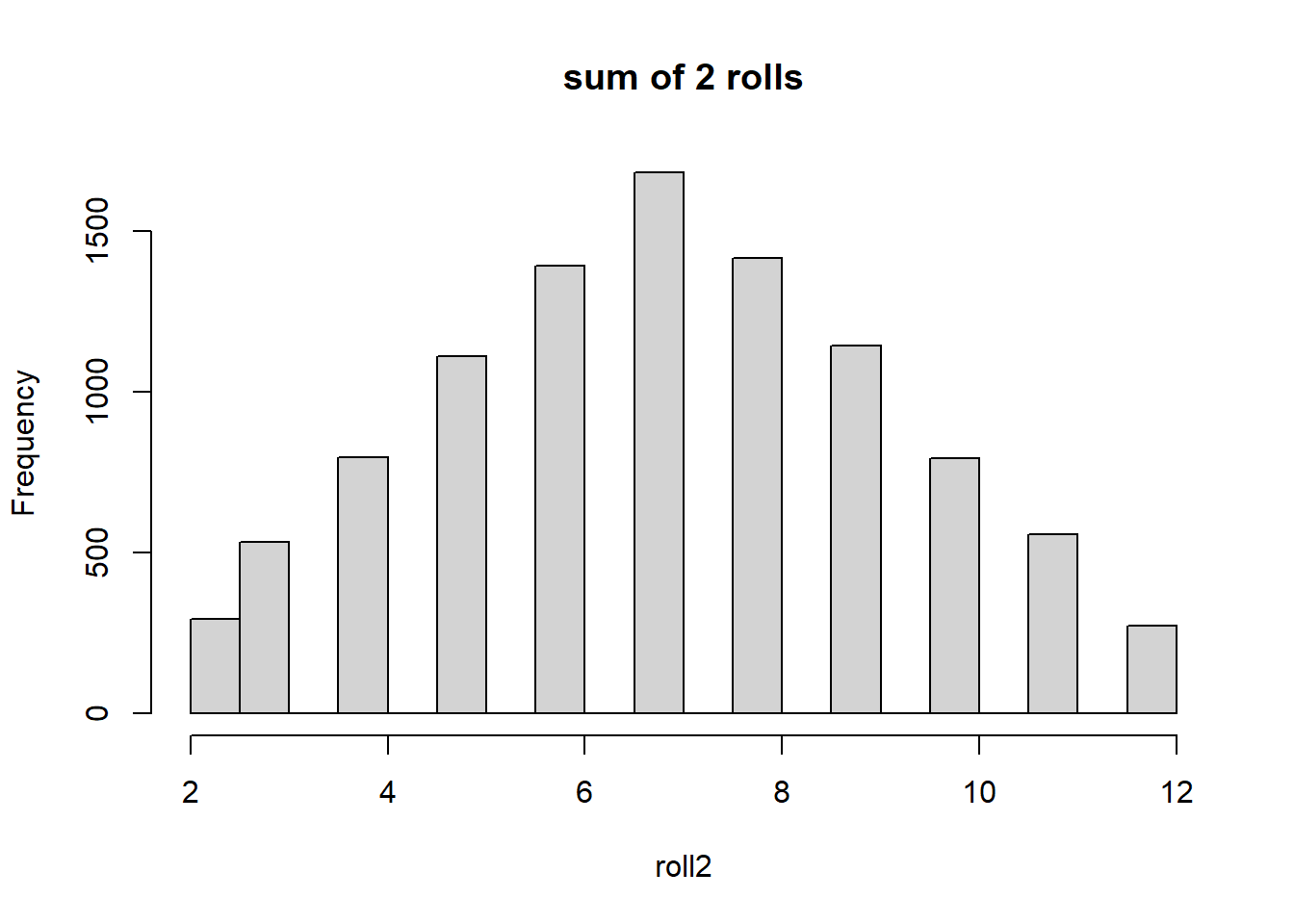

Similarly, we can plot the distributions of the sum of 3 and 4 dice rolls.

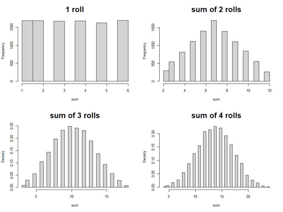
Do you notice something? As we sum up more dice rolls, the shape of the distributions starts looking more and more like a bell curve.

You get similar results if you count the number of heads/tails from multiple coin flips. Indeed, although we won’t get into the math of it, you can trust that the sum of many random events follows a normal distribution.

Now consider the blood pressure of a particular JCU student at this moment. What are some of the factors that could have affected this measure? Numerous, right? and each one of these factors is kind of random and can be considered a die roll.

Along the same line, many human physical and mental traits can be considered the joint result (sum) of numerous random events, which is why they tend to form a normal distribution.

4.2 What is a normal distribution?

Now can you tell which of the following curves are bell curves?

In fact, they are all bell curves, which begs the question of how bell curves are defined.

The normal distribution has a precise mathematical definition which we won’t get into. It’s definitely unimodal and symmetrical, but not all unimodal and symmetrical distributions are normal.

What really matter in this definition are the proportions. Consider how you can immediately recognize the picture of someone as a child or an adult, even if the sheer size of the picture stays the same. One important criterion we use, perhaps subconsciously, is the proportion of the head. Children have enormous heads compared to their bodies.

In the same vein, what the above 4 bell curves have in common are the propoprtions of their shoulders and tails etc. Indeed, what all normal distributions share in common is this: the same width always goes hand in hand with the same proportions. To be more specific, the same width (measured by standard deviation) always maps to the same % of cases, as illustrated here:

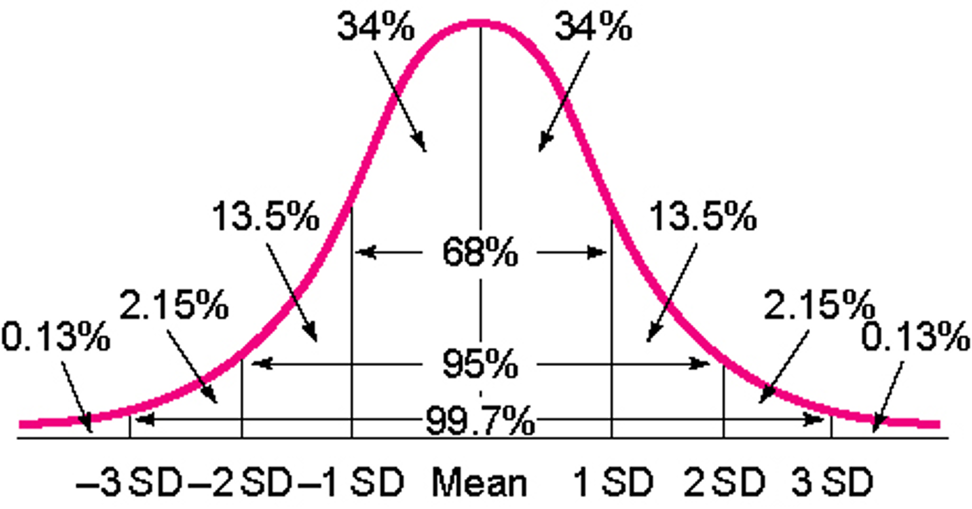
This defining feature of the normal distribution is laid out more precisely by the Empirical Rule.

The Empirical Rule

If a data set has an approximately bell-shaped distribution, then

approximately 68% of the data lie within one standard deviation from the mean, that is, in the interval $(\mu-\sigma, \mu+\sigma)$;
approximately 95% of the data lie within two standard deviations from the mean, that is, in the interval $(\mu-2\sigma, \mu+2\sigma)$;
approximately 99.7% of the data lies within three standard deviations of the mean, that is, in the interval $(\mu-3\sigma, \mu+3\sigma)$

Example 4.1

Meet Lu, an Olympic weight lifter. We recorded 50 of his snatches in the past 5 years. The mean is 170 kg (375 lbs), SD is 3 kg.

To predict how much he can snatch the next time, we can apply the Empirical Rule:

68% of the time, he would snatch within this range \[(\mu-\sigma, \mu+\sigma)=(170-3, 170+3)=(167,173)\]

95% of the time, he would snatch within this range \[(\mu-2\sigma, \mu+2\sigma)=(170-6, 170+6)=(164,176)\]

99.7% of the time, he would snatch within this range \[(\mu-3\sigma, \mu+3\sigma)=(170-9, 170+9)=(161,179)\]

Note that a big margin of error–give and take 9 kg–would raise the accuracy of our prediction, but it also tends to be less useful, e.g. to predict that tomorrow’s temperature will be between 20 and 120 degrees, I will certainly be correct, but it won’t be helpful. Whereas a more useful prediction, with smaller margins of error, is less likely to be accurate. To balance it out, we conventionally use the 95% interval, but it also depends on the context. When you hear about the margin of error in a national poll, it often means a 68% interval.

Example 4.2

The worship attendance at a church in Ohio was recorded for 209 consecutive weeks. From this approximately normally distributed data we get: $\mu=361.7$, $\sigma=58.5$

On any given day, what’s your estimate of this church’s attendance? Please give a specific number.
On any given day, what’s your estimate of this church’s attendance? Please give a range.
On Christmas’ day the church recorded an attendance of 490. Is this number unusual? Why?

Answer:

This specific number is what we call point estimate, and the best guess, of course, is the mean. I would round it to 362.
This range is what we call interval estimate. You can choose among any of the three kinds of intervals. But the most commonly used is the 95% interval: \[(\mu-2\sigma, \mu+2\sigma)=(361.7-2\times 58.5)(361.7+2\times 58.5)=(244.7, 478.7)\] And since we are talking about the number of people here, I would round it to (245, 479)
The attendance number of 490 is unusual since it is outside of my predicted range of (245, 479). Since this prediction should hold 95% of the time, an event that is outside of it must be pretty rare.

4.3 The z-score: How the normal distribution helps us making judgement

The last question of example 4.2 gives us a taste of what it involves to evaluate a number. When we say a number is particularly high or low, what we are really talking about is how likely it is for such a number to occur.

Let’s see if you can tell whether the following measurements are normal or abnormal:

A 27 degree (Celsius) day
An adult woman weighs 60 pounds.
Peter has an IQ score of 80.
A Will Smith movie that grossed $34 million.
The UK lost tens of thousands of tons of cargo every month during the early phase of WWII due to German submarine attacks.

I’m sure some of these numbers are meaningful to you. They may even make us emotional, such as the 60 lbs. Others can be meaningful immediately after translation. For example, if the 27 degree Celsius means nothing to you, then an 80 degree day would immediately bring back the summer in our minds. Still others, such as the IQ score of 80 and the $34 million gross for Will Smith, do not have quick translations and need more context.

If you know that the first Men in Black film grossed $441 million worldwide, you’d understand that the $34 million gross is a disaster for Will Smith.

For the IQ scores, though, we need more information. Even if I tell you that the average IQ is 100, it’s still not quite clear how low is 80. Surely not everyone below average is considered intellectually disabled. What we need to know is, on average, how much people differ from the average, i.e. the standard deviation.

Now if we are told that the standard deviation of the IQ distribution among the general population is 15, what do we know about Peter?

We can simulate a normal distribution of 10,000 IQ scores with $\mu=100$ and $\sigma=15$ in R, and find out where Peter is

iq=rnorm(10000,100,15)
hist(iq)
abline(v=80,col="red")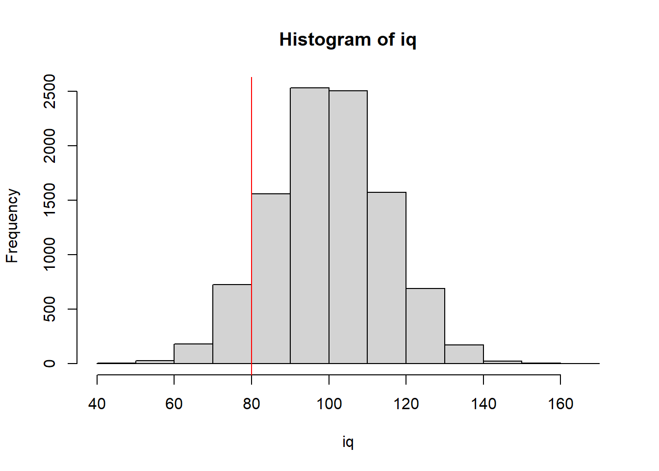

It looks like his ranking would be rather low, but perhaps not so low as indicating a disability.

Can we be more precise in evaluating this score? Yes. By converting this raw score of 80 into a z-score, we can actually get Peter’s percentil rank in the general population.

The z-score Formula

\[ z=\frac{x-\mu}{\sigma} \]

where $x$ is the number we are trying to interpret, and and are mean and standard deviation of this measurement’s distribution.

So now we can calculate a z-score for Peter: \[ z=\frac{80-100}{15}=\frac{-20}{15}\approx -1.33 \]

We can use a simple R function to convert this z-score to percentile rank:

pnorm(-1.33)

## [1] 0.09175914

Note that this result, 0.09175914, is a proportion. To turn it into a percentile rank, we must multiply it by 100. It’s also a good idea to round it to, say, 2 digits after the decimal point:

\[ 0.09175914\times 100 \approx 9.18 \] So Peter’s IQ score has a percentile rank of 9.18, meaning he is equal to or higher than approximately 9% of the population.

How to read a z-score:

The sign of the z-score tells us if the particular number is above or below the mean.
The absolute value of the z-score tells us how many standard deviation is this number away from the mean. if the absolute value of a z-score is at or above 2, it is considered quite rare. If it’s above 3, it’s very rare.

A couple more things about the z-score:

z-scores do not depend on metrics, which means they can be compared across different metrics!
z-scores and percentile ranks can be converted to each other when the distribution is roughly normal.

To convert a percentile rank to a z-score, the R function is qnorm, for example:

qnorm(0.09175914)

## [1] -1.33

4.4 Exercises

In the US, adult male heights are on average 69.1 inches (5’9.1) with a standard deviation of 2.9 inches. Adult women are on average a bit shorter and less variable in height with a mean height of 63.7 inches (5’3.7”) and standard deviation of 2.7 inches. Calculate your own z-score and percentile rank.
The mean of the IQ test is 100, standard deviation is 15. The cutoff for intellectual disability is 70. How many percentage of people would be screened as disabled?
Renee scored 87 on test 1 (mean = 90, SD = 3) and 89.5 on test 2 (mean = 92, SD = 5). Assume that higher score is better, on which test did she do better?
Answer the following questions using the dataset “StateData.sav”

The variable “TeenPreg” represents teen pregnancy rate in 2005 among girls 15-19 years old in each of the 50 states, and another variable, “GradPoor” represents graduation rate among economically disadvantaged students in 2010-11. For each of these variables, create a histogram, and find its mean and standard deviation.

Note: if you get “NA” as a result, it means that there are missing values in the data (NA = Not Available). To calculate the mean and standard deviation disregarding the missing values, use the following code:

mean(na.omit(TeenPreg)) 
sd(na.omit(TeenPreg))

Assuming the above distributions are normal, use their means and standard deviations to find the range for each of the variables that would include any given state 95% of the times.
Find the states that are outside of these intervals. What are their teen pregnancy rates and graduation rates among the economically disadvantaged? (Note: to save some work here, try sorting the variables with the command sort.)

Answer the following questions based on the results from two mental health screening measures in a cohort of adolescents in Texas. They include the CES-D 10 battery for depression screening and the Screen for Child Anxiety Related Disorders. Higher scores indicate higher levels of depression/anxiety. Both distributions are roughly normal. The means and standard deviations are given below:

	$\mu$ (Mean)	$\sigma$ (Standard Deviation)
Depression	9	3
Anxiety	8	2

For depression and anxiety respectively, find the range of score that would capture any given student 95% of the time.
Calculate the following students’ z-scores and percentile ranks for the depression test; based on the percentile ranks, explain their depression levels (high or low; normal or abnormal): Heather 14; Marc 9; Linda 6
Emily scored 12 on both tests, so it seems that she is above average on both measures, but which of her measurement is more severe, depression or anxiety? Why?
Consistent with protocol, scores equal to or above 12 on the depression battery indicate a positive screening (i.e. they got a red flag), whereas the cutoff for the red flag on the Anxiety battery is 11. Given these cutoffs, how many percentages of the adolescent population would be screened as positive on the two tests respectively?