Chapter 7 Hypothesis Tests
7.1 Independent and Dependent Variables–Recap
Example 7.1
Research Question: Do women make less money than men?
There are two main variables in this research question–income and gender. Which is the independent variable and which is the dependent variable?
This study implies that people’s incomes may depend on their gender to some degree. In any case, it’d be ridiculous to say that people’s gender depends on their incomes.
So, the variable that depends on the other one is the dependent variable. In this case, it’s income. The variables that does NOT depend on the other one is the independent variable. In this example, it’s gender.
In this class, we mainly deal with 3 types of research questions–prediction/correlation, group comparison, and causal inference. The following table may help you identify the independent and dependent variables in each case.
| Independent Var. | Dependent Var. | |
|---|---|---|
| Prediction | What the prediction is based on | What is to be predicted |
| Group Comparison | Group membership e.g. gender | What is being compared |
| Causal Inference | Cause | Outcome/Result |
7.2 Research Hypothesis and Null Hypothesis
When researchers conduct a quantitative research study, they typically already have a theory regarding their research question. This theory posits a general explanation of the causal connections between the facts. It is a story we tell to explain why there is variation. The goal of the research study is to test and update the theory.
A hypothesis is a testable prediction derived from the theory.
For example, before the battle of Midway during WWII, the US code breakers were able to decode some of Japanese radio messages. They noticed two letters, “AF,” appearing repeatedly in these messages. Based on their understanding of the Japanese strategies and the geography of the Pacific ocean, they believed “AF” stands for the Midway islands. This was their theory and they needed to prove it.
The US Navy code breakers contacted the Midway via the underwater secure cable and asked the Americans there to send a radio message to Hawaii, declaring falsely that they were running out of fresh water. They predicted/hypothesized that the Japanese would intercept this message and report it to their headquarters so the letters “AF” would appear again repeatedly in the Japanese radio message. This is a hypothesis. It is derived from the theory and it is directly testable.
And btw, the code breakers were right, and it was one of the keys of success for the US Navy during the battle of Midway.
Your ordinary educational researchers typically come up with hypotheses that are much less intricate than that. For example, my theory might be that 3rd graders need to practice reading in order to get good at it. Based on this theory, I may hypothesize that reserving a short period of class time for students to read independently and silently would raise their reading scores.
So a hypothesis is usually much more specific and actionable than a theory. It states a relationship between a specific independent variable (e.g. whether they use class time to read or not) and a dependent variable (e.g. the reading scores).
Research Hypothesis
The research hypothesis states the researcher’s belief.
Null Hypothesis
The Null hypothesis, regardless of what the researcher believes, always states that there is no relationship between the dependent and independent variables, or there is no difference between groups.
A hypothesis test always tests the null hypothesis.
Example 7.2
Research Question: is educational attainment related to income?
The Null Hypothesis is stated as
\(𝐻_0\): there is no correlation between educational attainment and income.
or
\(𝐻_0: r_{Ed, Income}=0\)
Research Question: do athletes have better work ethic than non-athletes?
\(𝐻_0\): There is no difference between athletes and non-athletes in terms of their work ethic.
or
\(H_0: \mu_{athlete} - \mu_{nonathlete}=0\)
7.3 Hypothesis Test–Step by Step
Remember the PPDAC cycle? The 5 letters represent the 5 steps in a hypothesis test.
Step 1 (problem): Raise the research question.
Step 2 (plan): State the Null Hypothesis (in order to come up with a testable hypothesis, we must already have a plan).
Step 3 (Data): Recruit a sample; take measurements of the sample.
Step 4 (Analysis): Analyze the data.
Step 5 (Conclusion): Draw a conclusion regarding the null hypothesis–reject or accept.
Example 7.3
Research question: are boys more likely to have ADHD than girls?
\(H_0\): There is no difference between boys and girls in their chances of having ADHD.
Collect evidence: Get a sample of children; record their gender and their ADHD diagnosis
Analyze the data.
Conclusion: based on the analysis result, we decide if this sample supports the null hypothesis.
7.3.1 What do we do when we “analyze the data?”
We have discussed the first 3 steps of hypothesis testing to various degrees in previous chapters. I would like to roughly explain the 4th step without getting into too much math.
What do we do when we analyze, say, the ADHD data of a group of children? Don’t we just compare the percentages of ADHD diagnoses among boys and girls? That sounds pretty easy. Why do we need to take a course in statistics to do that?
Well, we certainly do compare the percentages of ADHD diagnoses among boys and girls, but that’s not all we do in our data analysis.
Recall that, in inferential statistics, we use a sample to make inference about a larger population. This means that we are not extremely concerned with any tiny difference between this group of boys and girls. Instead, our fundamental question is, is the difference significant enough to make us believe that it is systematic and pervasive, and therefore may exist among other similar groups of boys and girls as well.
Example 7.3 Continued
Suppose we collected data for the boys vs. girls in ADHD question. In each of the following 4 scenarios, there is difference between boys and girls, but in which case(s) would you call the difference “significant?”
Scenario 1:
Boy ADHD rate = 20%, Girl ADHD rate = 10%
Sample size: 10 boys and 10 girls, i.e. 2 boys and 1 girl have ADHD
Scenario 2:
Boy ADHD rate = 90%, Girl ADHD rate = 0%
Sample size: 10 boys and 10 girls, i.e. 9 boys have ADHD and none of the girls has it.
Scenario 3:
Boy ADHD rate = 7%, Girl ADHD rate = 6%
Sample size: 100 boys and 100 girls, i.e. 7 boys and 6 girls have ADHD.
Scenario 4:
Boy ADHD rate = 7%, Girl ADHD rate = 6%
Sample size: 10,000 boys and 10,000 girls, i.e. 700 boys and 600 girls have ADHD.
Compare scenarios 1 and 2. In the first one, the difference between boys and girls doesn’t seem particularly striking. It could very well have been a small fluke. If we sample another 10 boys and 10 girls, how confident are we to see the same kind of difference again? Probably not very confident. In the second scenario though, the difference really stands out. If we randomly cast a net and would see 9 out of 10 boys having ADHD and none of the girls has it, it would certainly look like a problem that’s worth our attention, right? Can it be a fluke? Yes of course. But the chance of it being a fluke is much smaller than in scenario 1. What’s the chance that you flip a coin 10 times and get 9 heads?
Compare scenarios 3 and 4. The differences in ADHD rates are identical, but sample sizes are different. While the 7 boys and 6 girls in scenario 3 could be a fluke that is easily reversed–sample another 100 boys and 100 girls, we might get 6 boys and 7 girls with ADHD, the 700 boys vs. 600 girls in scenario 4 is much less likely to be reversible.
What does it mean to say a correlation/difference is significant?
To say a correlation/difference is significant means that it is unlikely to happen by chance, i.e. non-accidental.
The significance of the correlation/difference depends on:
How big the correlation/difference is;
How big the sample is.
So, in the data analysis stage of a hypothesis test, we analyze the significance of the correlation/difference, and this is how we do it:
First, a p-value is estimated which is the likelihood that the correlation/difference happened by chance.
Next, we compare the p-value with a pre-determined significance level (aka \(\alpha\), usually set at 0.05).
- If \(p<\alpha\), we conclude that the correlation/difference is significant, i.e. it is unlikely to have happened by chance.
- If \(p>\alpha\), we conclude that the correlation/difference is not significant, i.e. it is likely to have happened by chance.
p-value
P stands for probability, therefore it ranges from 0 to 1.
It is the likelihood that the observed difference/correlation happened by chance.
In other words, it is the probability that the null hypothesis is correct.
If you are rooting for your research hypothesis to be correct (usually we believe there is a real difference/correlation), that means that you want your p value to be small.
7.3.2 Conclusion
First of all, we don’t prove a hypothesis to be true or false in a hypothesis test. Recall that the hypothesis is usually about a general population and yet in a particular research study we only have access to a sample. It is not possible to prove something to be true or false in general with a mere sample. Even if we have access to the so-called “big data,” it is still impossible to prove something to be generally true or false for people in the past and in the future.
Instead of proving the hypothesis, we simply state, in the conclusion stage, that the null hypothesis is rejected or accepted. If the particular study stands the test of peer review and is allowed to be published, our conclusion will be counted as a piece of evidence to be reckoned in the long run.
For example, no one has ever been able to prove that smoking causes lung cancer in any single research study. It has become common knowledge after the accumulation of evidences over decades of intense research:
In many studies, the incidence of lung cancer is so much higher among smokers than non-smokers that it’s unlikely to be due to chance.
We see the same results repeated in studies after studies that it’s beyond reasonable doubt.
Conclusion of a Hypothesis Test
The level of significance (\(\alpha\)) is usually set at 0.05 (this is related to the fact that confidence intervals are usually built at the level of 95%).
Occasionally, researchers also use \(\alpha=0.01\) or \(\alpha=0.1\)
If \(p<\alpha\), reject the null hypothesis;
if \(p>\alpha\), accept the null hypothesis.
7.4 One-Sample t Test
We will now illustrate the steps and principles of hypothesis testing with a one-sample t test.
One-sample t tests are used when we compare a single group with a population and try to decide if the group belongs to the population.
In the last exercise problem of Chapter 3, we looked at the heights of 12 US presidents during the TV era. We can now add President Biden to this dataset who is 72 inches tall.
According to data published by the Centers for Disease Control and Prevention (CDC) , the average height for American men 20 years old and up is 69.1 inches. Obviously no one is able to measure the height of all adult men living in the US, but the population mean can be reasonably well estimated by a carefully drawn sample.
The research question is, are presidents taller than the general male population, in other words, do we prefer taller people to be our presidents?
The null hypothesis is that there is no diference between the US presidents and the general US male population in their heights, in other words, the US presidents belong to the general population in terms of their heights.
\[H_0: \mu_{presidents}=69.1\] We will adopt \(\alpha=0.05\) for this analysis.
Next, we enter the data and carry out the one-sample t test:
presidents=c(70.5,72,76,71.5,72,69.5,73,74,74,71.5,73,75,72)

t.test(presidents, mu = 69.1)
##
## One Sample t-test
##
## data: presidents
## t = 7.0238, df = 12, p-value = 1.387e-05
## alternative hypothesis: true mean is not equal to 69.1
## 95 percent confidence interval:
## 71.52490 73.70586
## sample estimates:
## mean of x
## 72.61538“mean of x,” 72.61538, is the mean of our sample of presidents.
“df,” degree of freedom, gives away the sample size: sample size = df + 1 = 13
“95 percent confident interval,” [71.52490, 73.70586], can be understood in this way: there is a 95% chance that the next president we have after Joe Biden will be between 71.5 and 73.7 inches tall. Of course, the next president could be a woman, and in that case, the height expectation won’t be applicable, but we know how hard it is to elect a female president–the overall chance is definitely small.
Lastly, “p-value = 1.387e-05.” Recall scientific notation we introduced in the first class?
\[1.387e-05=0.00001387\] Therefore \(p<\alpha\), and we reject the null hypothesis.
So the difference between the heights of the group of 13 presidents and that of the general population is unlikely due to chance, that is to say, the difference is significant. The US presidents are significantly taller than the average American adult males.
7.5 Type I and Type II Errors
Just like how the jury members never saw the crime, or how the doping committee members never saw the athletes taking drugs, statisticians don’t see lung cells turning into cancer under the influence of smoking.
In a hypothesis test, we make dichotomous decisions, either rejecting or accepting the null. As said earlier, we cannot prove the hypothesis to be true or false, which means our decisions are always prone to errors. This is not only because what is true for the sample is not necessarily true for the general population, but also since our understandings of the science could be limited and even our measurement instruments could be error-prone.
7.5.1 Type I Error
If an athlete tested positive for doping, it means that he/she is believed to have doped. If someone tested positive for Covid-19, it means that he/she is believed to have Covid. If these test results are incorrect, we call this type of error a false positive. False positive is also known as type I error.
When someone tests positive for something it means that he/she differs from the normal population. Therefore, another way to understand type I error is that we are rejecting the null hypothesis by mistake.
Since we won’t reject a null hypothesis unless \(p<\alpha\), it means we cannot possibly commit a type I error unless \(p<\alpha\). Setting \(\alpha\) very small is something we can do to control the chance of type I error. The level of significance (\(\alpha\)) is the maximum acceptable probability of making a type I error.
7.5.2 Type II Error
When someone actually has Covid but tests negative, it’s called a false negative—type II error.
In other words, we make a type II error when we accept the null hypothesis by mistake.
The probability of making a type II error is denoted as \(\beta\).
| Truth: Athlete doped | Truth: Athlete did not dope | |
|---|---|---|
| Committee’s decision: Athlete doped | Correct Decision: doper is caught! | Type I Error. Athletes: Do we alpha pay da bill? |
| Committee’s decision: Athlete did not dope | Type II Error. Competitors: We beta get some dope, II! | Correct Decision: Innocent athlete maintained integrity! |
7.5.3 The relationship between type I and II errors
As mentioned earlier, \(\alpha\) is a lever we have to control type I errors. Is it possible to make sure that we never make any type I errors? Absolutely. Just set \(\alpha=0\), which means we will never reject any null hypothesis. This way we won’t make any type I error.
The problem with doing so is that it will certainly increase our chance of making type II errors.
The following plots illustrate the relationship between type I and II errors.
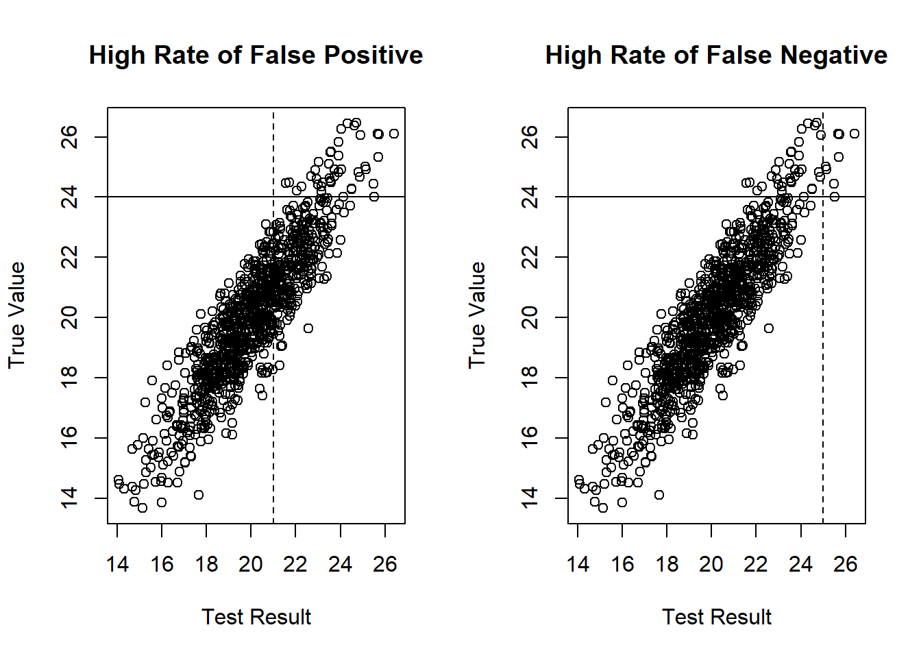
The vertical dashed line is the cutoff for the test results. The horizontal solid line is the actual threshold of the true value of the underlying trait. The dots ending up in the lower right quadrant are the false positives, and those in the upper left are the false negatives.
When we move the vertical dashed line to the right, it is equivalent of maneuvering \(\alpha\) to make it smaller, and we can thus reduce the false positives. But then the false negatives will inevitably increase.
The upshot is that it is not possible to eliminate both type I and II errors. But it is possible to find an optimal balance between them.
In practice, we don’t always need to consider this issue as a novice data analyst, since we can just follow the convention of setting \(\alpha=0.05\). Sometimes though we may come across research studies that set their \(\alpha\) at 0.1 or 0.01. So it’s important to understand the consequences of choosing a larger or smaller \(\alpha\).
7.6 Exercises
7.6.1 Identify the independent and dependent variables
- Is test anxiety a good predictor of test scores?
- Does having a disability affect a child’s decision of attending public or private schools?
- Does financial assistance improve the symptoms of mentally ill patients?
- Does a country’s institutional corruption increase its citizen’s tendency to lie?
- Are boys more likely to drop out of high school than girls?
7.6.2 We’d like to research the idea that praising children for their effort makes them more resilient. Please lay out the steps for the hypothesis test.
7.6.3 Which ones of the following are appropriate null hypotheses?
A. \(𝐻_0\): praising children for effort makes them more resilient. B. \(𝐻_0\): praising children for effort does not make them more resilient. C. \(𝐻_0\): The 400 children praised for effort would score higher on the resiliency test than the other group not praised for effort. D. \(𝐻_0\): In general, children praised for effort would score equally high on a resiliency test than those not praised for effort.
7.6.4 True or False
- The p-value is a number that ranges from -1 to 1.
- P in the p-value stands for probability.
- The p-value is the likelihood that the relationship we saw in the sample is absolutely real.
- Large p-values, such as 0.8, indicates that the observed outcome is highly likely to be an accident.
7.6.5 Decimals and percentages
- .0007= ____%
- 0.1%=_____
- 0.745=_____
- 0.01=_____
- 0.01%=_____
7.6.6 The scientific notation
- 2.734e+4 =
- 1.324e-5 =
- 7.32e-3 =
Use the scientific notation to represent these numbers: 1) 7380 = 2) 0.00246 =
7.6.7 Investigators wish to study the question, “do blondes have more fun?”
- What is the null hypothesis in this question?
- What would be a type I error in this case?
- What would be a type II error?
- If one investigator uses a .05 level of significance (i.e. alpha) in investigating this question and another one uses .001 level of significance, which would be more likely to make a type I error?
7.6.8 Type I and II Errors
Based on a random sample of teenage girls from the north and south, researchers concluded that there is no significant difference between north and south in teen pregnancy rates. But others question this finding. They are suggesting that it may be a type __ error.
An experiment shows that eating grapefruit can help you lose weight. But later a design flaw of the experiment was found–those who ate grapefruit regularly also happened to exercise more than the no-grapefruit group. The original conclusion could be a type __ error.
In the above question, one researcher uses an alpha of 0.05, another researcher uses an alpha of 0.01. The first researcher, compared to the second:
A. Is more likely to make the type I error B. Is more likely to make the type II error C. Is more likely to make errors. D. Is less likely to make errors.
7.6.9 One-sample t tests
7.6.9.1 Please test the hypothesis that a middle-aged man in UK has had 7 sexual partners on average using the dataset “sexual.partners.sav.”
- State the Null Hypothesis (in words or in an equation).
- Carry out the data analysis in R. Copy and paste your codes here. Note: After reading in the data, we need to first select a subset of the dataset that only includes men. Use the following codes to accomplish this:
Male.sample=subset(NickNameofDataset, sex=="m")
attach(Male.sample)- Copy and paste the output from R. Interpret the p-value, the 95% confidence interval, the degrees of freedom, and the sample mean.
- Do you reject or accept the null hypothesis?
- Has this sample had more or less than 7 sexual partners on average?
7.6.9.2 The adult American men have an average height of 69.1 inches. We would like to find out if men in our class are taller or shorter than the national average using our class survey data.
- State the Null Hypothesis (in words or in an equation).
- Carry out the data analysis in R. Copy and paste your codes here. Note: After reading in the data, we need to first select a subset of the dataset that only includes men. Use the following codes to accomplish this:
survey.male=subset(NickNameofDataset, gender=="M")
attach(survey.male)- Copy and paste the output from R. Interpret the p-value, the 95% confidence interval, the degrees of freedom, and the sample mean.
- Do you reject or accept the null hypothesis?
- Are men in our class taller or shorter than the national average?
7.6.9.3 The average American has visited 12.5 states, according to Ipsos polls. We would like to find out if our class has travelled more or less than the national average using our class survey data.
- State the Null Hypothesis (in words or in an equation).
- Carry out the data analysis in R. Copy and paste your codes here.
- Copy and paste the output from R. Interpret the p-value, the 95% confidence interval, the degrees of freedom, and the sample mean.
- Do you reject or accept the null hypothesis?
- Has our class travelled more or less than the national average?
7.6.9.4 The adult American women have an average height of 63.7 inches. We would like to find out if women in our class are taller or shorter than the national average using our class survey data.
State the Null Hypothesis (in words or in an equation).
Carry out the data analysis in R. Copy and paste your codes here. Note: After reading in the data, we need to first select a subset of the dataset that only includes women. Use the code given in some of the exercise problems above and make the necessary changes.
Copy and paste the output from R. Interpret the p-value, the 95% confidence interval, the degrees of freedom, and the sample mean.
Do you reject or accept the null hypothesis?
Are the women in our class taller or shorter than the national average?
7.6.9.5 Proteins in energy bars
The labels on a particular brand of energy bars claim that each bar contains 20 grams of protein. We have collected a random sample of 31 energy bars from a number of different stores to represent the population of this brand of bars available to the general consumer. The data are listed in the following table
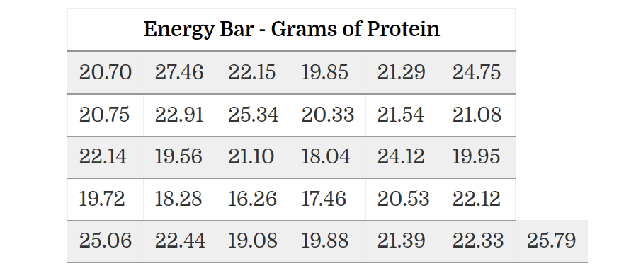 Enter this data in R and carry out a one-sample t test to test the hypothesis that the labels are generally correct. State the null hypothesis; produce the necessary statistics; and draw your conclusion. Please make sure to include your R code and output.
7.6.9.6 Many cities in the US are known for their crimes. The average violent crime rate per 100,000 in the US in 2012 was 693, including homicide, assault, rape, sexual assault, and robbery. The dataset “crimeInCity.sav” records crime rates for a group of cities. Please test the hypothesis that cities have more violent crimes than the national average using this data.
- State the Null Hypothesis (in words or in an equation).
- Carry out the data analysis in R. Copy and paste your codes here.
- Copy and paste the output from R. Interpret the p-value, the 95% confidence interval, the degrees of freedom, and the sample mean.
- Do you reject or accept the null hypothesis?
- Do cities have more or less violent crimes than the national average?