Chapter 10 Paired T Test
So far, we have learned the following types of hypothesis tests:
One-sample t test: To compare a sample with a single number
ANOVA: To compare multiple groups on a quantitative measure
\(\chi^2\) Test: To compare multiple groups on a categorical measure
Correlation: Relationship between two quantitative measures
In this chapter, we’ll learn yet another type of hypothesis test–the paired t test, aka matched t test or paired-sample t test.
10.1 When do we use paired t test?
In education and many other fields, it’s often useful to compare a before and an after measure, such as:
Did life quality improve after marriage counseling?
Did depression level decrease after therapy?
Did strength improve after training?
Did test score improve after using a curriculum?
The t test for matched (paired) samples is used when each individual in the data is measured twice (e.g. pretest and posttest), and we want to compare the two measurements.
Occasionally it is also used to compare means of two groups of people provided that they are paired, e.g. comparing the average number of hours spent on house chores by husbands and their wives.
If we use ANOVA to test the before-and-after effect, we lose sight of the fact that the before and after measurement come from the same individuals. As a result, our test would lose power—-some subtle but significant differences might not be picked up.
10.2 How to carry out paired t test?
Example 10.1
Step 1. Research Question:
Did students’ reading performance improve from kindergarten to first grade?
Step 2. State Null hypothesis
\[ H_0: \mu_k=\mu_1\] We will also set \(\alpha=0.05\).
Step 3: Data
library(foreign)
ecls=read.spss("ecls.sav",to.data.frame =TRUE)
attach(ecls)
Step 4: Analysis
First, take a look at the variables and their labels:
View(ecls)The reading scores from the spring of kindergarten and first grade are named “c2rrscal” and “c4rrscal.”
Get some descriptive statistics for each of these variables:
summary(c2rrscal)## Min. 1st Qu. Median Mean 3rd Qu. Max.
## 12.00 28.00 34.00 35.61 40.00 85.00summary(c4rrscal)## Min. 1st Qu. Median Mean 3rd Qu. Max.
## 16.0 50.0 59.0 58.8 69.0 89.0Now let’s visualize this comparison:
boxplot(c2rrscal,c4rrscal,names=c("Kindergarten","First Grade"))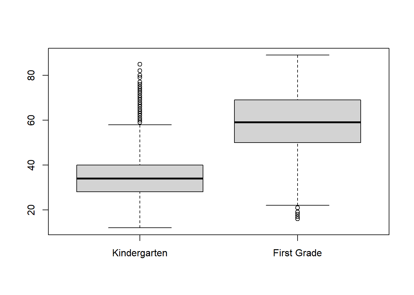
The boxplots show that, on average, students have made a lot of improvement over that year. The first year distribution also seems to be more spread-out than the kindergarten. This indicates that the achievement gap is growing as well.
Note that in the above code, we put a comma between the variables. Remember sometimes we put a ~ between the variables? When should we use which?
Well let’s try it out:
boxplot(c2rrscal~c4rrscal)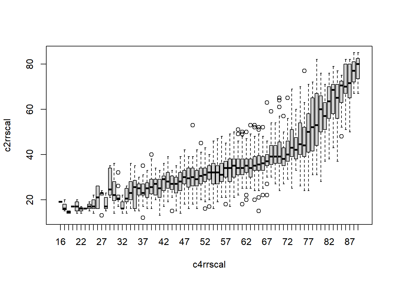
Did youWould you be able to make sense of this plot? If not, it’s probably not the right plot.
Now let’s get the p-value for the paired t test
t.test(c2rrscal,c4rrscal,paired=TRUE)##
## Paired t-test
##
## data: c2rrscal and c4rrscal
## t = -131.14, df = 2576, p-value < 2.2e-16
## alternative hypothesis: true difference in means is not equal to 0
## 95 percent confidence interval:
## -23.53413 -22.84073
## sample estimates:
## mean of the differences
## -23.18743Step 5: Conclusion
Since \(p<\alpha\), we reject the null hypothesis. Students’ reading scores in first grade are significantly higher compared to their own scores in kindergarten.
10.3 Difference and Relationship
People sometimes get confused about paired t test and correlation, since they often deal with the same variables.
In a correlation between kindergarten and first grade reading scores, kindergarten score is the independent variable; first grade score is the dependent variable.
Let’s look at the correlation coefficient and the scatterplot:
cor.test(c2rrscal,c4rrscal)##
## Pearson's product-moment correlation
##
## data: c2rrscal and c4rrscal
## t = 56.906, df = 2575, p-value < 2.2e-16
## alternative hypothesis: true correlation is not equal to 0
## 95 percent confidence interval:
## 0.7287496 0.7629845
## sample estimates:
## cor
## 0.7463604plot(c2rrscal,c4rrscal,xlab="Kindergarten",ylab="First Grade")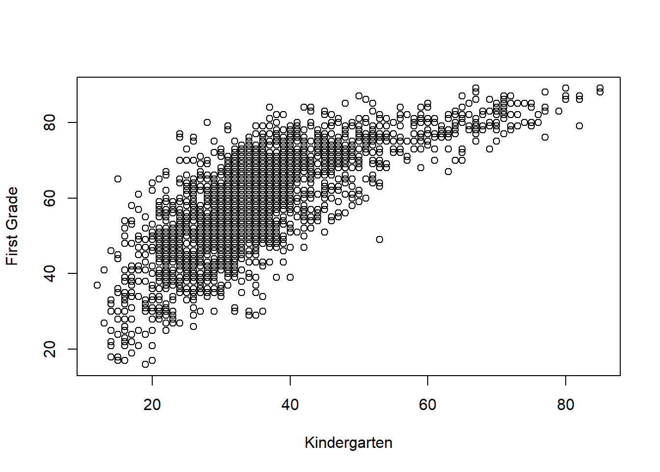
The correlation coefficient shows that there is a strong and significant (since \(p<\alpha\)) correlation between kindergarten and first grade scores.
The scatterplot visualizes this correlation.
It means that those who were good readers in kindergarten are very likely to be good readers in first grade. As well, those who were poor readers in kindergarten are most likely poor readers in first grade.
In a paired t test comparing kindergarten and first grade scores, the two variables are actually neither independent nor dependent variables. They are simply two measurements to be compared. We can also say that test score is the dependent variable while grade level (or time) is the independent variable, since grade level defines the groups to be compared.
10.4 Exercises
10.4.1 Choose the appropriate kind of hypothesis test for the following research questions
Is there a gender achievement gap in reading in the first grade?
Are those who scored lower in kindergarten still lag behind in second grade?
Do girls grow faster than boys in reading from kindergarten to first grade? (this one can be tricky, we haven’t learned the right kind of test for it but there is still something we can do.)
10.4.2 Carry out a paired-sample t test for each of the following research questions using the dataset “ecls.sav.”
Both teacher and parents rated their students’ in terms of their eagerness to learn. Do parents rate their own children higher than the teachers? State the null hypothesis, get some descriptive statistics for both measurements, visualize the comparison, get the p-value, and draw your conclusion.
Run a paired t test comparing children’s internalizing and externalizing behavior ratings. The variable name for internalizing behaviors is “t1intern,” it includes behaviors that direct problematic energy towards self, such as behaviors associated with depression and anxiety. The variable name for externalizing behaviors is “t1extern.” It includes behaviors that direct problematic energy towards others, such as lashing out at others and other disruptive or aggressive behaviors.
State the null hypothesis for this test.
What are the respective means of children’s internalizing and externalizing behavior ratings? Create a side-by-side boxplot to illustrate the comparison.
What is the p-value? What does it mean?
State your conclusion of this hypothesis test.
Given that higher ratings means the behaviors are more frequent and more problematic. Which is the dominating behavioral problems among this age group of children, internalizing or externalizing?
- Compare internalizing and externalizing behavior ratings among boys. Follow the above steps. To select boys from the dataset, use this code:
male=subset(data.name, gender=="male")
attach(male)
- Compare internalizing and externalizing behavior ratings among girls. Follow the above steps.