Chapter 8 Analysis of Variance
Recall that one-sample t test is a type of hypothesis test. We use this test when we only have one group, hence “one-sample,” and we test if the mean of the population represented by this group is equal to a known number.
More frequently in educational or other behavioral research, we don’t have a known number in our hypotheses. Instead, we have 2 or more groups to be compared to each other. The type of hypothesis test used when we compare several groups on a quantitative measure is called Analysis of Variance, aka ANOVA. Note that in an ANOVA, the dependent variable is quantitative, and the independent variable (which group the participant is in) is categorical.
8.1 Why is it called Analysis of Variance?
ANOVA is used to compare group means. To be more accurate, it is used to compare the means of the populations represented by the groups.
But why is it called Analysis of Variance?
This is because the variance of each group plays an important role in the mean comparison. Let’s look at a couple of examples.
8.1.1 Comparing Tarons and Americans.
The Taron is an ethnic group in the Himalayan foothills of Myanmar, who is on the verge of extinction. They have been referred to as the “East Asian pygmies.” Like the Pygmies of Central Africa and other parts of Southeast Asia, the Tarons are very small. Their adult women have an average height of 4 foot and 7 inches.
According to a 2018 report from the Centers for Disease Control and Prevention (CDC), the average height among all American women, age 20 and up, is 5 foot 4 inches.
It is harder to find out about standard deviations, but according to one demographic study, the global standard deviation of women’s heights ranges from 2.1 to 3.2 inches. We will use the high end of this interval, 3.2, as the standard deviation for both Taron and American.
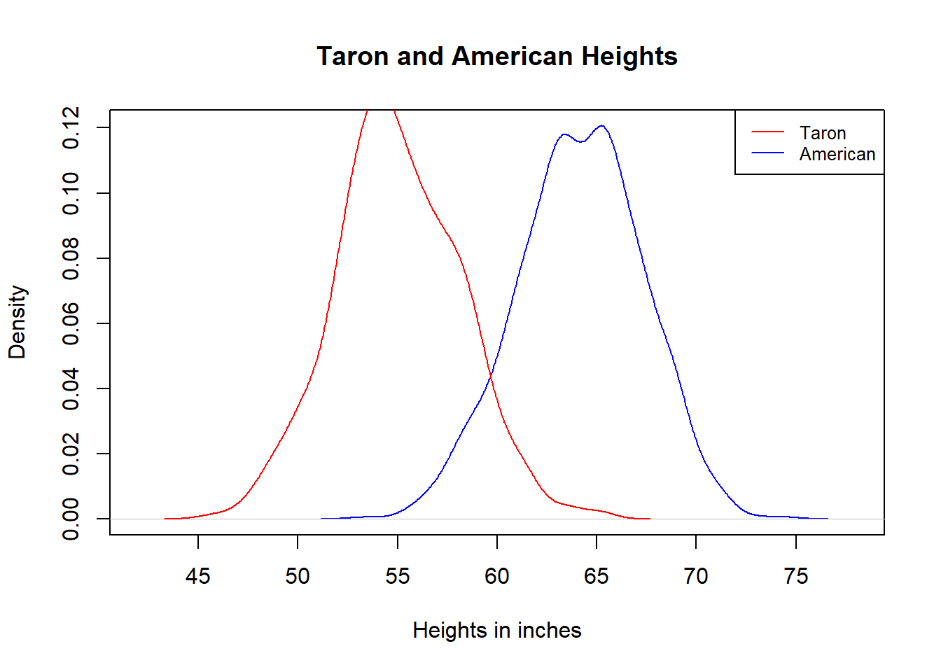
Note that the mean difference, \(5'4''-4'7''=9''\), is much larger than the standard deviation of each group, 3.2 inches. This means that each of the two distributions, once visualized, is slim enough to show the gap between them.
Below is a visualization of 2 simulated distributions based on the actual means and standard deviations and the assumption that both are normal. The two bell curves are indeed clearly separated. If we have the data, the height difference will certainly prove to be significant.
8.1.2 Comparing American crocodiles and American alligators.
Reptiles differ from us mammals in that they would keep growing larger after reaching sexual maturity, so their adult lengths have a much larger standard deviation.
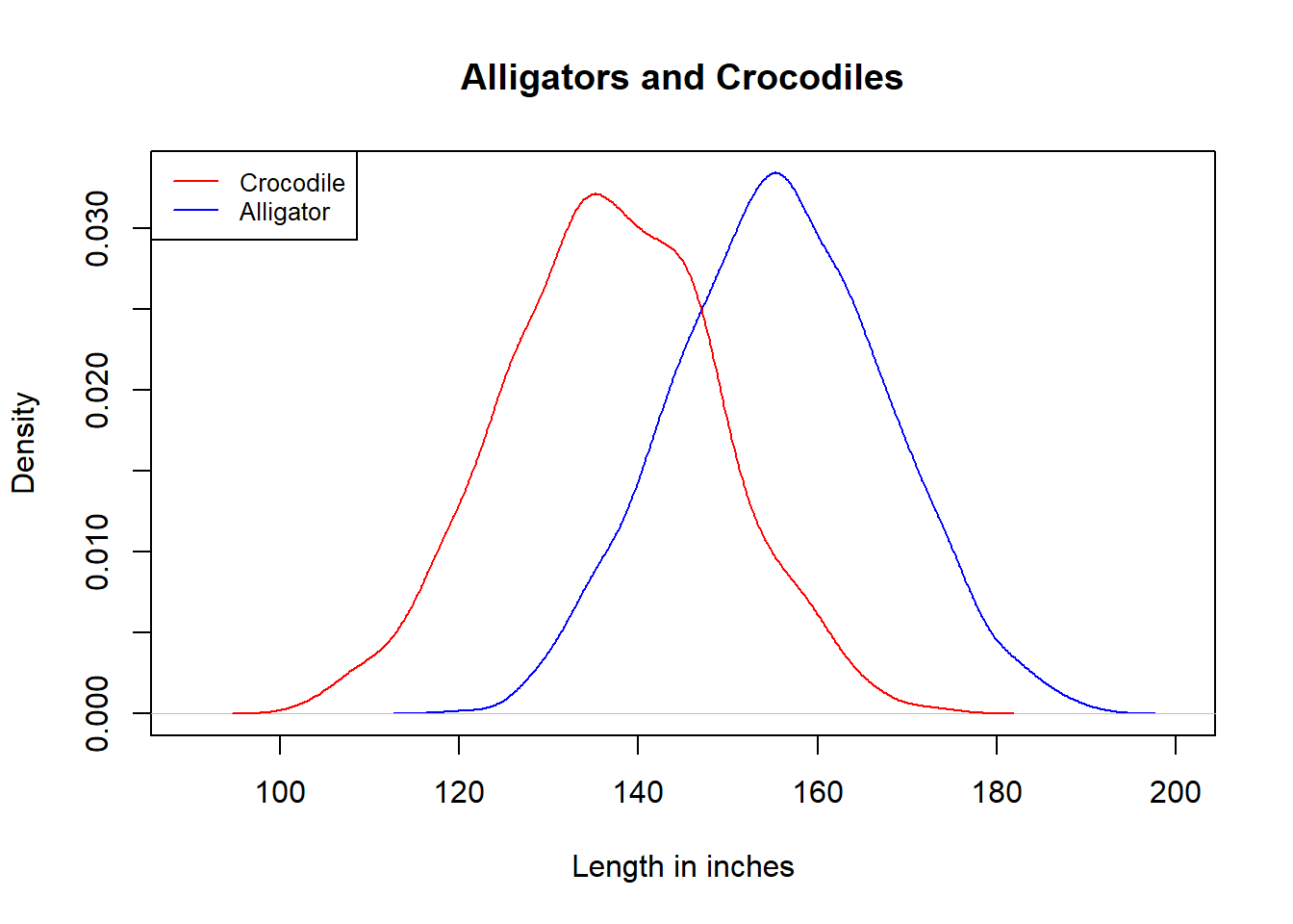
According to one estimate, adult male American alligators have an average length of 13 ft, while mature males American crocodiles are on average 11 foot 5 inches in length. The mean difference between them is much larger than that of the Tarons and American women.
But American alligators and crocodiles each has a standard deviation of about 1 foot in length. With such wide distributions, the gap between them actually looks a bit smaller and less obvious than the Taron-American comparison, as shown below.
The upshot is that, when comparing group means, we use the standard deviations within each group as a measurement unit.
Recall in chapter 2.4, when we talk about the change of risk, we don’t just do \(P_2-P_1\), instead we measure this difference against the original risk: \(\frac{P_2-P_1}{P_1}\)
Also in chapter 4.3, when we talk about how much a particular score deviates from the population mean, we don’t just do \(x-\mu\), instead we measure the difference against the standard deviation of the population distribution: \(\frac{x-\mu}{\sigma}\)
The same thing is happening here. The sheer difference among group means does not give us a sense of how extraordinary it is. It needs to be measured against how much individuals differ from each other within the group.
8.2 Doing Analysis of Variance
Since ANOVA is just another type of hypothesis tests, we follow the same steps as those of the one-sample t test.
Example 8.1
For this example we will use the dataset “ecls.sav.” “ecls” stands for Early Childhood Longitudinal Study. It is a very rich dataset. I encourage you to take a look at the variables and play with them.
Our specific question is whether there is a gender achievement gap in reading as early as the start of kindergarten.
The relevant variables are “c1rrscal” which is the reading score in the fall of kindergarten, and “gender.”
Step 1. Research Question: Do boys and girls differ in their reading scores in the fall of kindergarten?
Step 2: Null hypothesis
\(H_0\): there is no difference between boys and girls in terms of their reading scores in the fall of kindergarten.
or
\(H_0: \mu_G=\mu_B\)
We should also set \(\alpha\) at this stage: \(\alpha=0.05\). If you skip this, it means you have adopted the conventional value for \(\alpha\), which is 0.05.
Step 3: Data
We don’t need to collect the data. It is given to us. So let us just import it into R:
Don’t forget to set working directory first.
library(foreign)
ecls=read.spss("ecls.sav", to.data.frame=TRUE)
attach(ecls)
View(ecls)
Step 4: Analysis
Before we proceeds to get the p-value, it is always a good practice to get some descriptive statistics: how many boys and girls do we have in this dataset? What are their average reading scores in fall kindergarten? What are their standard deviations?
R has a convenient function to help us get these information. It is stored in a package that we need to download using the following code. But you only need to do it once.
install.packages("FSA")Once you installed the package, you don’t need to do it again. But everytime you use it, you need to bring it to the forefront:
library(FSA)Now we can use the function “Summarize” in this package. Note that the dependent variable precedes the independent variable in the parenthesis.
Summarize(c1rrscal~gender)## gender n mean sd min Q1 median Q3 max
## 1 male 1280 24.20703 9.623569 11 18 22 28 79
## 2 female 1297 25.56978 9.651166 11 19 24 30 81It looks like girls do have a slight advantage over boys in reading. The difference is not that big compared to the group standard deviations. It’s always a good idea to visualize the comparison:
boxplot(c1rrscal~gender)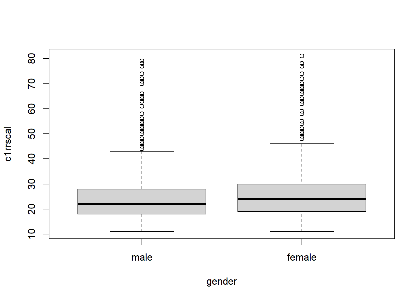
The gender gap is visible, but doesn’t seem substantial. Is it statistically significant? Let’s get the p-value. Again, DV first, IV next.
oneway.test(c1rrscal~gender)##
## One-way analysis of means (not assuming equal variances)
##
## data: c1rrscal and gender
## F = 12.881, num df = 1.0, denom df = 2574.7, p-value = 0.0003381Step 5: Conclusion
Since \(p<\alpha\), we reject the null hypothesis. Girls score higher than boys in their reading test of fall kindergarten, and the difference is significant.
In the previous example, the difference between boys and girls is really not that big, especially measured against the group standard deviations. Why did it turn out to be significant?
Remember there is another factor that has a heavy influence over the p-value–the sample size. Suppose, instead of 2577 boys and girls, we had 50 boys and girls in the data. Would we still get such a small p-value for their comparison?
Let’s try it out.
With the following code, I first took a small sample that includes a random draw of 50 rows from the original ecls data. I then carried out the analysis using the small sample.
small.sample=ecls[sample(1:2577,50),]
Summarize(small.sample$c1rrscal~small.sample$gender)
## small.sample$gender n mean sd min Q1 median Q3 max
## 1 male 27 23.44444 7.536237 11 19.5 22 28.5 44
## 2 female 23 24.52174 7.470363 13 22.0 23 27.5 46oneway.test(small.sample$c1rrscal~small.sample$gender)##
## One-way analysis of means (not assuming equal variances)
##
## data: small.sample$c1rrscal and small.sample$gender
## F = 0.2562, num df = 1.000, denom df = 46.872, p-value = 0.6151The output shows that, although the mean difference between boys and girls is slightly larger than that of the big dataset, p is now larger than , so the difference is no longer statistically significant.
Why? Because a sample size of 50 is not enough evidence. Considering that the mean difference is so small, had we drawn a different sample of 50, it would be conceivable that the difference might changed or even reversed.
Whereas a sample size of 2577 is a lot of evidence. Even if the mean difference is small, it’s hard to imagine that it would be annihilated or reversed with a different sample.
When group difference is significant in an ANOVA, it means
The mean difference is big enough compared to the standard deviations within each group.
The sample size is also decent.
8.3 Exercises
In the dataset “ecls.sav,” the variable “s2kpupri” records if a student went to public or private schools.
8.3.1 Run an ANOVA comparing reading scores from spring of first grade between public and private school students.
- What are the independent and dependent variables?
- How many students are there in public and private schools and what are their mean reading scores?
- State the null hypothesis for this test.
- What is the p-value? What does it mean?
- State your conclusion of this hypothesis test.
- Is there an achievement gap between public and private school students? Which type of school has higher achievement?
- Create a side-by-side boxplot to illustrate your conclusion.
But wait, does higher student achievement mean that the teachers and administrators in that school do a better job? Are we so sure that it’s the school that caused that achievement? This is what led to the next question, how do public and private school students compare to each other when they just entered school?
8.3.2 Run an ANOVA comparing reading scores from fall of kindergarten between public and private school students.
- How many students are there in public and private schools and what are their mean reading scores?
- State the null hypothesis for this test.
- What is the p-value? What does it mean?
- State your conclusion of this hypothesis test.
- Is there an achievement gap between public and private school students in the beginning of kindergarten?
- Create a side-by-side boxplot to illustrate your conclusion.
8.3.3 Correlation and causation
Strictly speaking, when we say that a school is good, we don’t necessarily mean that it has high-achieving students, instead we mean that the school (i.e. teachers, principal, and other personnels) contributes to great student growth. Now, based on your findings from the above two analyses, do you think we have solid evidence that one type of school has contributed more to student growth than another type of school? Why?