Chapter 5 Correlation
5.1 Plotting the relationship between 2 Variables
Take a look at the following two plots. In the left plot, height is measured in inches, and weight is measured in pounds. In the right plot, exercise is the average number of hours people work out in a week. Weight is again measured in pounds. What do these two plots tell us?
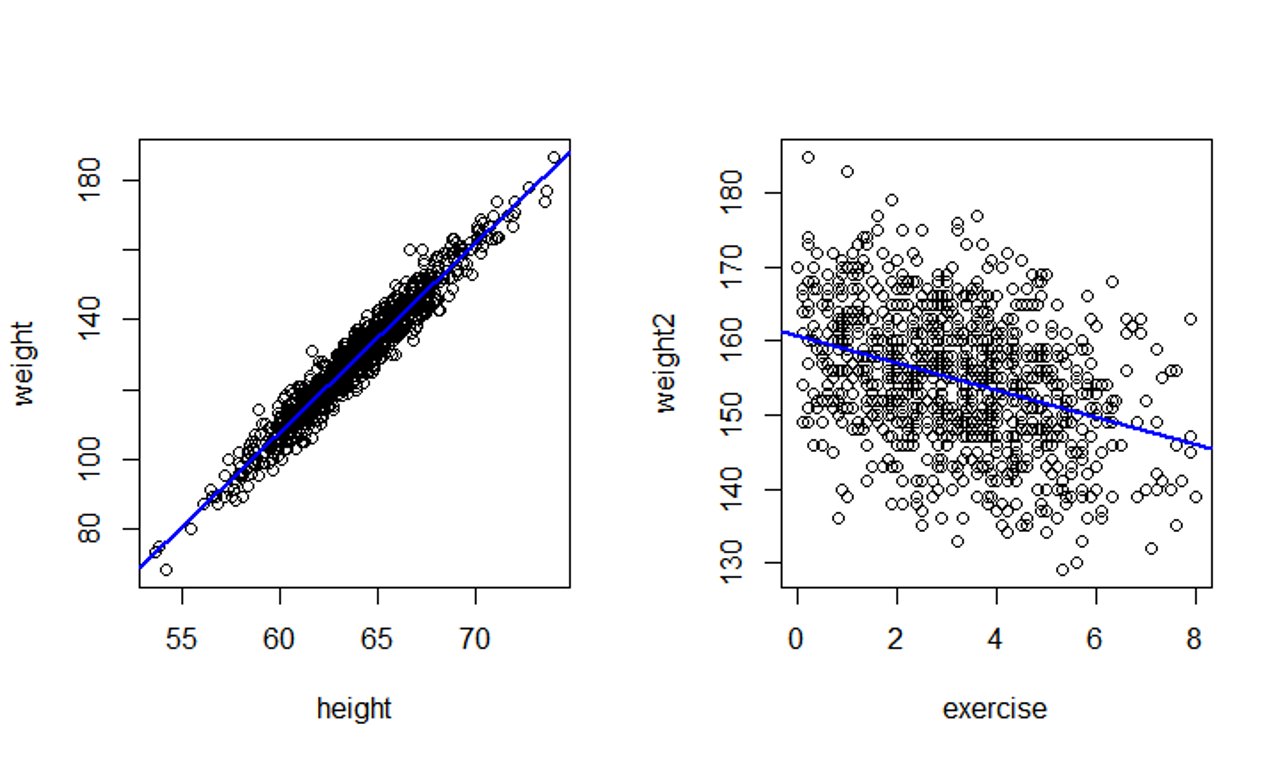
Scatterplots 1 and 2
Recall that the plots we have learned to create so far, histograms, bar plots, pie charts, etc., only handles one variable at a time. But the pictures you see above represent two variables in a single plot.
Also note that the variables represented here are all quantitative.
Plotting the relationship between 2 quantitative variables
This kind of plot that represents two quantitative variables with two axes are called scatterplots.
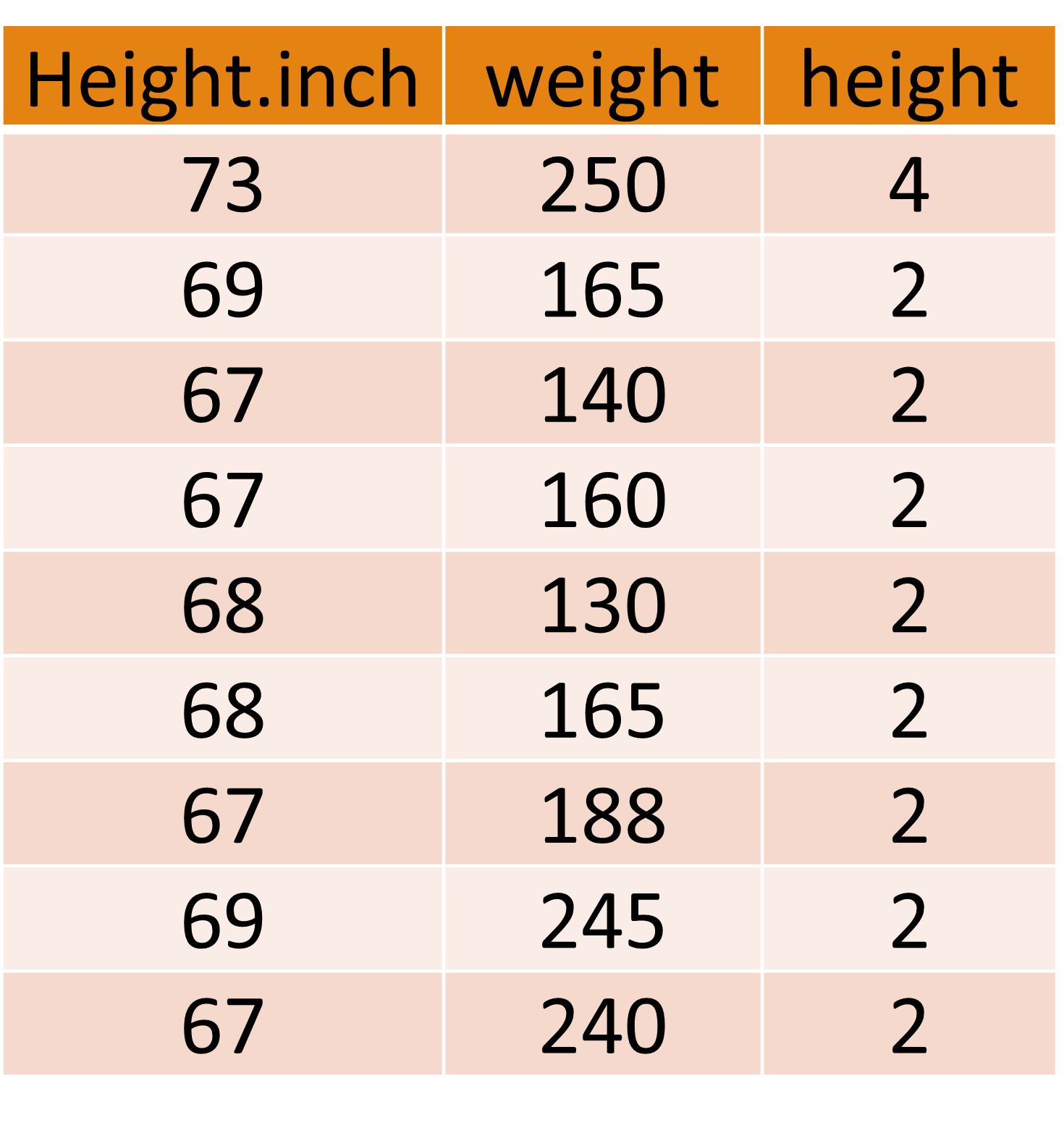
Now take a look at scatterplot 3 below and a snapshot of its data.
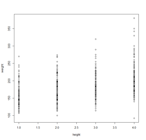
Why does this scatterplot look so weird?
If you examine the data carefully, you’ll see that the “height” variable used in the scatterplot is not really a measurement of people’s heights. It consists of values 1, 2, 3, and 4. These people were divided into 4 groups based on their height. So “height” in this particular dataset is a categorical variable.
We do get a sense that people in group 4 are on average taller than those in group 3, and group 3 is taller than group 2, etc. Still, the comparison is not very clear.
Instead, the picture below, which puts 4 boxplots side by side to each other, tells us the same thing as scatterplot 3, and is much easier to read.
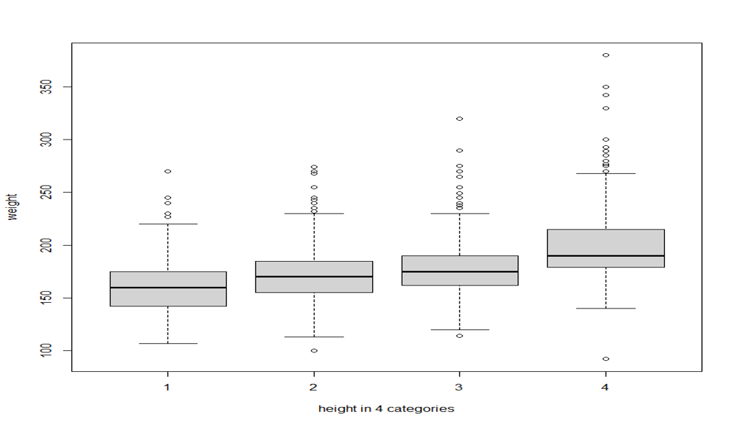
Side-by-side boxplots
Plotting the relationship between a quantitative and a categorical variable
It is usually not a good idea to plot the relationship between a quantitative variable and a categorical variable with a scatterplot. Side-by-side boxplots would be a better choice.
5.2 Correlation
In statistics, the relationship between two variables are often called correlation.
In the scatterplots below, each dot represents a country. “Lit_fema” in the left plot is the % of adult females in a given country who are literate. “fertility” in the right plot is the average number of births the women in a particular country give in their lifetimes. And in both plots, the vertical axes, “lifeexpf,” is the life expectancies of women in each country.
Can you explain the correlations visualized in these plots?

5.3 What kind of data are suitable for correlation?
Can we produce a scatterplot for the correlation between female literacy rate and male literacy rate of these countries?
Can we produce a scatterplot for the correlation between female literacy rate of one group of countries (say, European) with another group of countries (e.g. Asian)?
To have a correlation, we need two measurements from each case in the dataset.
5.4 Independent and Dependent Variables
Correlation is extremely useful in the sense that it tells us if we can use one variable to predict another.
SAT scores are used to predict freshman year GPA in college.
T4 cell count were used to predict HIV/AIDS in 1980s before an HIV test was available
High blood pressure is used to predict many medical conditions
What is used to make the prediction is called the predictor, or the Independent Variable.
What is being predicted is called the outcome, or the Dependent Variable.
5.5 How to create a scatter plot
First of all, we need two variables, both of them quantitative.
By convention, the independent variable is put on the x-axis; the dependent variable, on the y-axis.
Use our class survey data as an example. Suppose I have a pet theory that people who watch a lot of movies also tend to have travelled more, perhaps because they want to see the places they learned about in the movies, or perhaps watching a lot of movies simply means you have a lot of spare time. In any case, I’d like to use the variable “movies” to predict the variable “states.” So “movies” would be the independent variable, and “states” would be the dependent variable.
First, we need to load the data. Don’t forget to set your own working directory.
survey=read.csv("ED101surveyfall21.csv",header=TRUE)
attach(survey)
## The following objects are masked from survey (pos = 8):
##
## edMajor, gender, height, movies, statesMake sure we know how the variable names are spelled:
names(survey)## [1] "height" "gender" "edMajor" "states" "movies" "dogCat"Now we can produce the scatterplot:
plot(movies, states)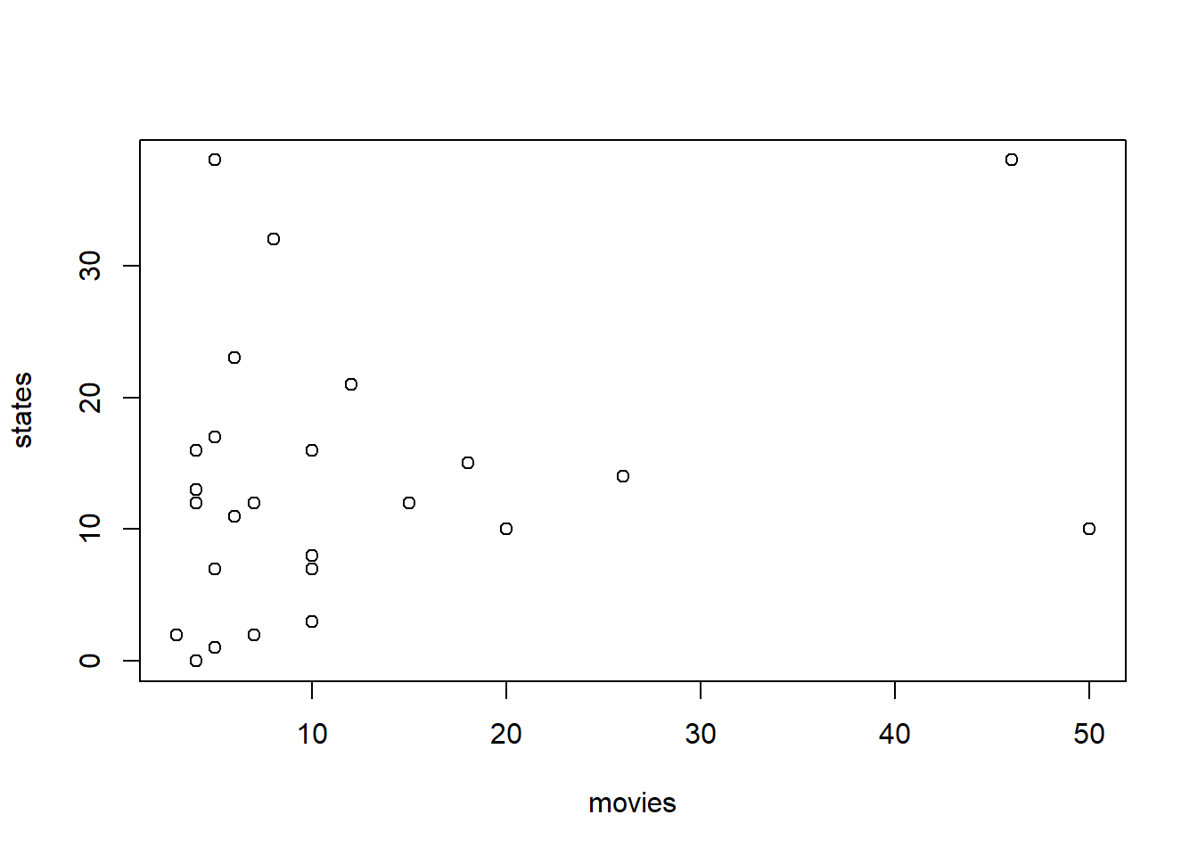
To add labels to the axes and a title to the plot:
plot(movies, states, xlab="Number of movies watched over break", ylab="Number of states visited", main="Survey Data from ED 101 Fall 2021")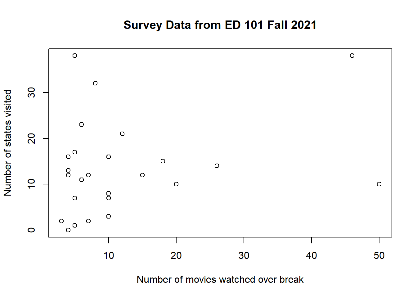
5.6 How to Read a scatterplot
Among the following correlations plotted, can you tell which are positive, which are negative, which are strong, which are weak?

We have a positive correlation when the two variables tend to change in the same direction.
We have a negative correlation when the two variables tend to change in different directions.
It’s probably clear that the upper middle plot above is a stronger correlation than the lower right one. What does it mean to be a stronger correlation? In the upper middle plot, as X goes up, Y is almost certainly going up as well. While in the lower right plot, as X goes up, Y is very likely to go up, but there is now a wider margin of uncertainty about where Y could be.
So the strength/magnitude of a correlation is the likelihood that X and Y change in accordance with each other.
The upper right plot shows the strongest possible correlation–as X changes, there is absolutely no uncertainty as to how Y would change.
The upper left plot shows a slightly weaker correlation–as X goes up, Y very likely to go down, although there is a bit of uncertainty about it.
The direction of a correlation is NOT relevant to its strength. A negative correlation can be strong, while a positive correlation can be weak.
5.7 The Correlation Coefficient, aka Pearson’s r
The correlation coefficient is an index to express the direction and strength of the relationship. It is bounded between -1 and 1 for any pair of variables.
The sign of the correlation coefficient indicates the direction of the correlation.
The absolute value of the correlation coefficient indicates its strength.
To find out the correlation coefficient of a pair of variables, use the following code:
cor.test(movies, states)##
## Pearson's product-moment correlation
##
## data: movies and states
## t = 1.3355, df = 23, p-value = 0.1948
## alternative hypothesis: true correlation is not equal to 0
## 95 percent confidence interval:
## -0.1419005 0.5998206
## sample estimates:
## cor
## 0.2682723The number that appears below “cor” is the correlation coefficient (Pearson’s r).
Here’s a rough rule of thumb to interpret the strength of r:
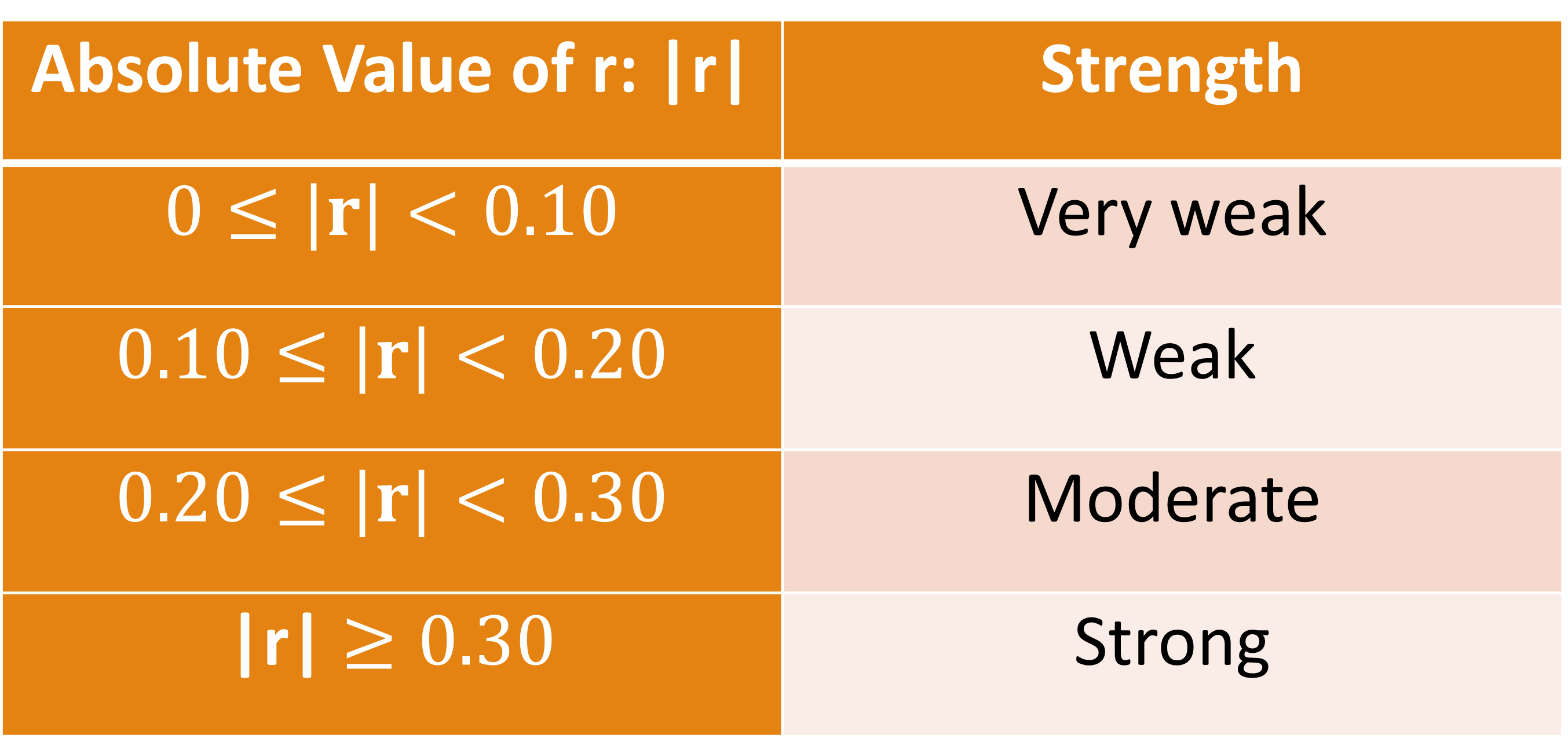
And, of course, values of 1 or -1 indicates a perfect (strongest possible) correlation.
Another useful number in the output is “df.” This number plus 2 is equal to the number of pairs we have in the data. So, in this case, there are 25 people in this class that provided usable data for both variables.
The “95 percent confidence interval” is a margin of error around the correlation coefficient. A wider margin, like this one, marks the extent of our ignorance/uncertainty about this relationship. Why are we still ignorant about the relationship between numbers of movies watched and states visited? Because we really don’t have a lot of data–25 pairs is a paltry size.
We’ll talk about the “p-value” in a couple of weeks.
5.8 What the correlation coefficient does and does not mean
5.8.1 r is not the slope
The correlation coefficient is an index to express the degree of relationship.
The correlation coefficient tells us whether it is possible to predict one variable based on the other, but it does NOT tell us how to make that prediction.
Example 5.1
Is the following statement true or false?
Given a correlation coefficient of 1 between X and Y, a score of 32 on X must be accompanied by a score of 32 on Y.
Answer: it is false.
Why?
In the following correlation, which is perfect, a score of 32 on X is indeed accompanied by a score of 32 on Y.
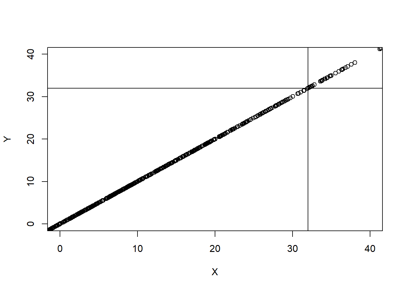
However, in the following two correlations colored red and orange, which are both perfect as well, a score of 32 on X is NOT accompanied by a score of 32 on Y.
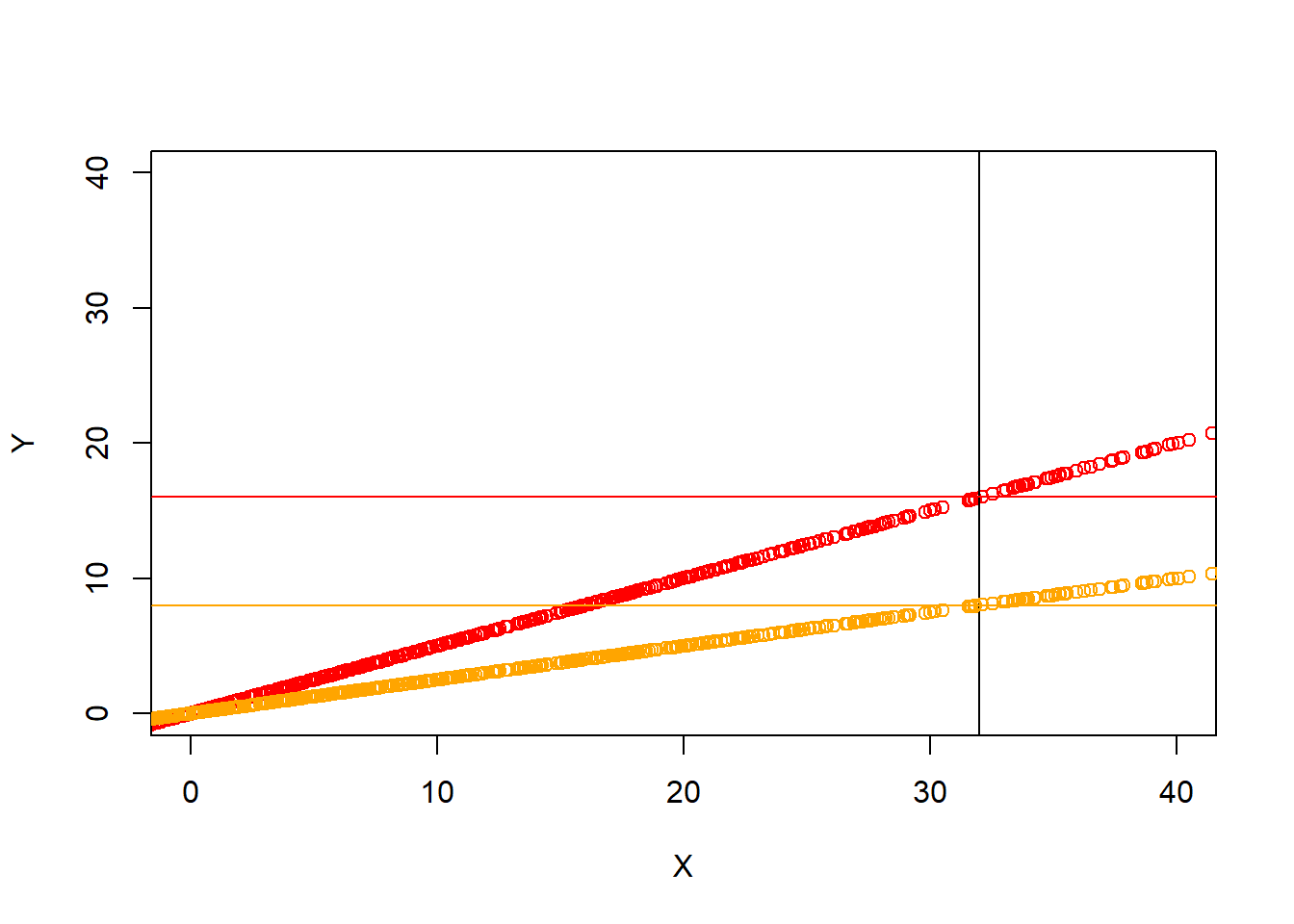
Remember, in the scatterplot, r shows up only as the tightness of the dots clustering around the invisible straight line. It has nothing to do with how steep that slope is.
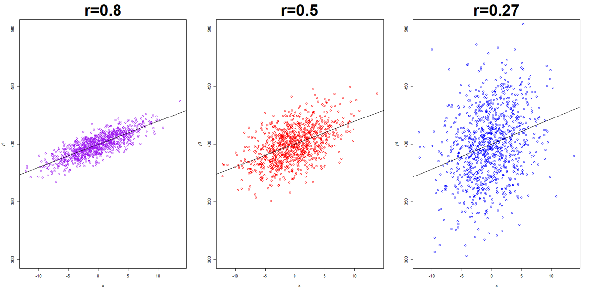
The following 3 scatterplots have identical upward slopes, and only differ in their tightness:
5.8.2 r only represents linear relationship
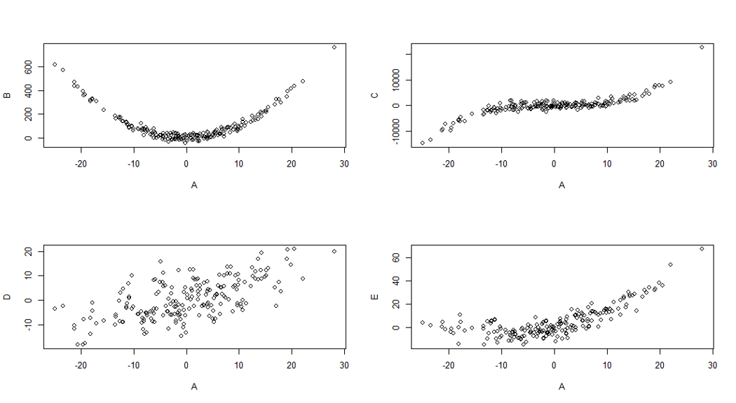
Non-linear correlations can be strong, too. But this strength is not picked up by r very well.
5.8.3 r could be unduely influenced by outliers
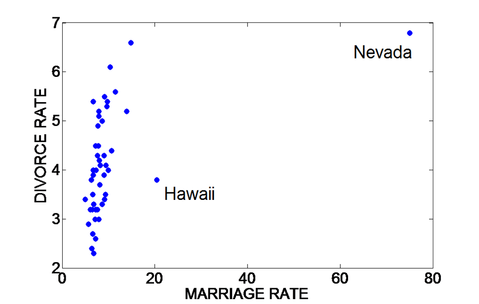
Sometimes when we just look at r, we get an impression that the correlation is not very strong, but when looking at the scatterplot, we realize the correlation is stronger than what r represents, it is just skewed by some outliers.
The upshot: whenever possible, take a look at both the statistic and the plot.
5.9 Exercises
5.9.1 The lowest magnitude of correlation shown below is:
0.65
–0.33
–0.85
0.45
5.9.2 Most of the examinees who score below the mean on Test 1 also scored below average in Test 2; the correlation between the two tests appears to be:
Positive
negative
near zero
d.1.0
5.9.3 If the coefficient of correlation between X and Y is found to be -0.98, which of the following would be indicated?
- X and Y are closely related
- X and Y are unrelated
- X and Y are perfectly related
- Y is a result of X
5.9.4 Given r (correlation coefficient)= 0.50 between X and Y, it follows that:
- Smaller X’s tend to be associated with smaller Y’s
- one-half of the Y values are less than the associated X values
- one-half of the X’s are less than the associated Y’s
- one’s standing on Y is about one-half that of his standing on X
5.9.5 Interpret the meaning of each of the following correlation coefficients (you can do so after the examples, or feel free to use your own language if you could try to stay close to the interpretations provided here):
Examples
The correlation between 3rd grade reading scores and 6th grade reading scores is 0.8.
Interpretation: This is a strong positive correlation. It means that children who have higher reading scores in the 3rd grade are very likely to have higher reading scores in the 6th grade as well.The correlation between adult height and IQ scores is 0.06. Interpretation: There is practically no correlation between adult heights and IQ scores. It means that tall people are equally likely to have high IQ as short people.
1). The correlation between scores on a reading test and an IQ test is 0.78.
2). Ratings of students on good citizenship and on aggressiveness show a correlation of -0.56.
3). The correlation between weight and sociability is 0.02.
5.9.6 Play with the dataset called “wvs” (world value survey).
Choose a pair of quantitative variables that, according to you, have some sort of relationship with each other (note: please do not use the pairs that are already used in class).
1). List the names of these variables. What do they mean?
2). Obtain some descriptive statistics (measures of central tendencies and variability) for each.
3). Create a scatterplot for the two variables. Copy and paste here.
4). Obtain the correlation coefficient (Pearson’s r) and interpret it.