Chapter 3 Describing a Quantitative Variable

3.1 Plotting the Distribution

We have learned how to create a histogram and a boxplot. Here’s another way to visualize quantitative data: stem-and-leaf plot

Open data:

library(foreign)
tv=read.spss("TV.sav", to.data.frame=TRUE)
attach(tv)

Get variable names:

names(tv)

## [1] "TVtime"

Create stem-and-leaf plot:

stem(TVtime)

## 
##   The decimal point is 1 digit(s) to the right of the |
## 
##    0 | 077902236778
##    2 | 01200333333
##    4 | 00444479455
##    6 | 057077
##    8 | 2018
##   10 | 2900
##   12 | 
##   14 | 0
##   16 | 5

3.2 Measures of Central Tendency

Get mean and median:

mean(TVtime)

## [1] 49.96

median(TVtime)

## [1] 42

Your turn: How would you get the mode?

Get the percentiles i.e. values corresponding to certain percentile ranks

• what is the 25th percentile, i.e the amount of TV time that is at the 25th percentile rank?

quantile(TVtime, 0.25)

##   25% 
## 20.25

• what is the 75th percentile, i.e the amount of TV time that is at the 75th percentile rank?

quantile(TVtime, 0.75)

##   75% 
## 69.25

• We can also get both percentiles at the same time

quantile(TVtime, c(0.25, 0.75))

##   25%   75% 
## 20.25 69.25

Get the percentile ranks:

Find out the percentile rank of the kid who watched 30 mins of TV

sort(TVtime) #sort the variable 

##  [1]   0   7   7   9  10  12  12  13  16  17  17  18  20  21  22  30  30  33
## [19]  33  33  33  33  33  40  40  44  44  44  44  47  49  54  55  55  60  65
## [37]  67  70  77  77  82  90  91  98 102 109 110 110 140 175

You can count that there are 17 kids who have TV time less or equal to 30, out of 50 in total, so the percentile rank is

17/50

## [1] 0.34

If you don’t want to count, you can do this

a=sort(TVtime) #name the sorted variable so you can use it later
length(a) #find out the total number of people there (the length of the vector)

## [1] 50

which(a==30) #find out the ranking position for value 30

## [1] 16 17

The above numbers lead to the same percentile rank: \(\frac{17}{50}\)

3.3 Measures of Variability/Dispersion

Get the five-number summary

summary(TVtime)

##    Min. 1st Qu.  Median    Mean 3rd Qu.    Max. 
##    0.00   20.25   42.00   49.96   69.25  175.00

Remember boxplot? The 3 bars in the box and the 2 bars at the end of the whisker are the five-number summary:

boxplot(TVtime)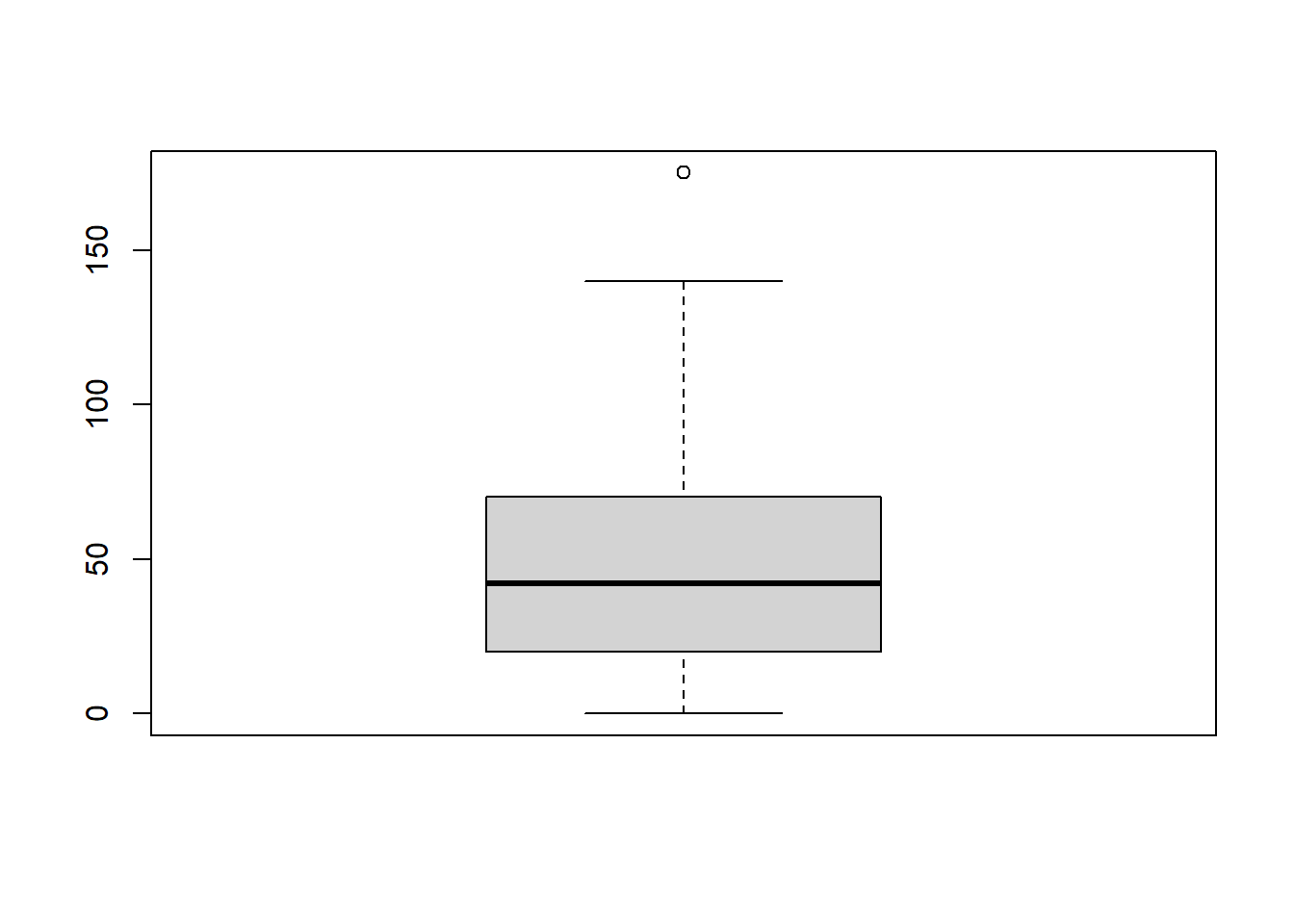

Range (\(Max-Min\))

max(TVtime)-min(TVtime)

## [1] 175

IQR (Inter Quartile Range: \(Q_3-Q_1\) or \(Q_U-Q_L\))

s.tv=summary(TVtime)
s.tv[5]-s.tv[2] #s.tv is a vector of 6 numbers, we are telling R to subtract the 2nd number (1st quartile) from the 5th number(3rd quartile)

## 3rd Qu. 
##      49

Standard Deviation is the most commonly used measure of variability/dispersion.

3.4 Standard Deviation

3.4.1 How to Calculate Standard Deviation

Suppose 5 different high school teachers are asked to grade the same essay, here are the scores they gave out of 100: 72, 65, 74, 81, 92. Following are the steps it takes to calculate the standard deviation of this distribution.

Step 1. The mean \[\mu=\frac{\sum x}{n}=\frac{(72+65+74+81+92)}{5}=\frac{384}{5}=76.8\]

To do this in R:

a=c(72,65,74,81,92)
mean(a)

## [1] 76.8

Step 2. Deviations

\[x-\mu=\begin{array}{c} 72-76.8\\ 65-76.8\\ 74-76.8\\ 81-76.8\\ 92-76.8 \end{array} =\begin{array}{c} -4.8\\ -11.8\\ -2.8\\ 4.2\\ 15.2 \end{array}\]

in R:

a-mean(a)

## [1]  -4.8 -11.8  -2.8   4.2  15.2

Step 3. Squared Deviations

\[(x-\mu)^2=\begin{array}{c} (-4.8)^2\\ (-11.8)^2\\ (-2.8)^2\\ (4.2)^2\\ (15.2)^2 \end{array}=\begin{array}{c} 23.04\\ 139.24\\ 7.84\\ 17.64\\ 231.04\end{array}\]

in R:

(a-mean(a))^2  # ^2 means take this number to the power of 2, i.e. square it

## [1]  23.04 139.24   7.84  17.64 231.04

or, the following gives the same result and might be easier to understand

dev=a-mean(a)
dev^2

## [1]  23.04 139.24   7.84  17.64 231.04

Step 4. Variance (mean of squared deviations)

\[\sigma^2=\frac{\sum (x-\mu)^2}{n}=\frac{23.04+139.24+7.84+17.64+231.04}{5}=83.76\]

in R:

mean(dev^2)

## [1] 83.76

or

dev.sq=dev^2
mean(dev.sq)

## [1] 83.76

Step 5. Standard Deviation (square root of the variance)

\[\sigma=\sqrt{\sigma^2}=\sqrt{83.76}\approx9.15\]

in R:

variance=mean(dev.sq)
sqrt(variance)

## [1] 9.152049

All the above 5 steps can be boiled down to 2 lines of code in R, although you might find the steps above easier to process, they are equivalent to the following:

a=c(72,65,74,81,92)
sqrt(mean((a-mean(a))^2))

## [1] 9.152049

Actually, R allows you to skip the calculation altogether, and get the variance or standard deviation directly:

a=c(72,65,74,81,92)
var(a) # var is the command that produces the variance

## [1] 104.7

sd(a) # sd is the command that produces the standard deviation

## [1] 10.2323

You probably noticed that the variance and standard deviations produced by the var and sd functions are different from what we calculated by hand.

This is because what we calculated is literally the variance/standard deviation of those five people, whereas what the R functions produce are the variance/standard deviation of a big population of which those five people form a random, representative sample.

In any case, the difference between the two camps is noticeable because we only have 5 data points, a small n as they say. When n increases to, say 50, the difference would be barely noticeable. And the datasets that we deal with usually have much bigger n.

3.4.2 What does the standard deviation mean?

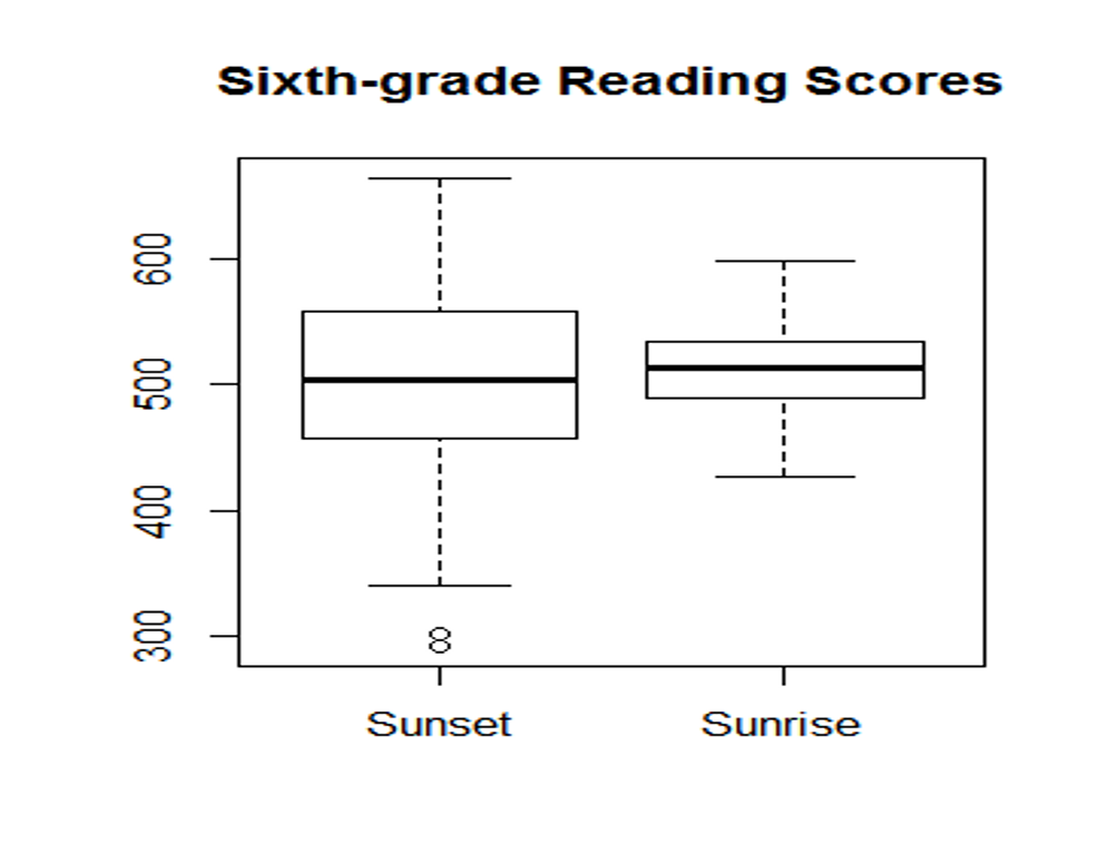
Since standard deviation is a measure of variability, a bigger standard deviation means bigger, well, variability, i.e. people are more different from each other. Here are the reading score distributions of 6th graders in two schools. If you happen to teach 6th grade language arts, where would you prefer to teach?

Here’s another hypothetical example: suppose we have results from a large-scale survey about European citizens’ attitudes towards refugees, higher scores indicating more positive attitudes. France and Germany have the same mean, but France has a much bigger standard deviation. If you are a refugee, where would you seek asylum?

You see that a larger standard deviation can mean more uncertainty, or less predictability, and uncertainty is something that has a powerful effect on our daily lives.

Now consider the effects of two types of drugs on lowering blood pressure as illustrated below. If you are a physician, which drug would you recommend to your patients?

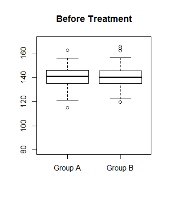
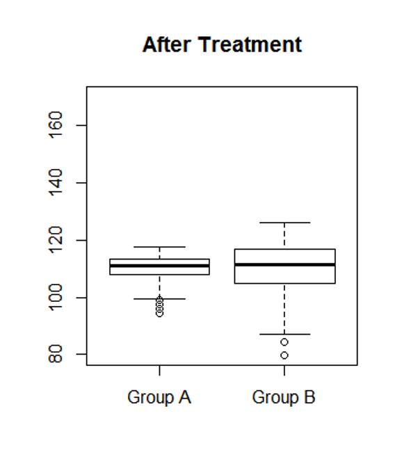
This example shows that a larger standard deviation can also mean less consistency or less reliability.

All the above examples involve groups of people, but even a single individual can have a standard deviation. How?

With repeated measurement.

Think about your favorite athlete. If you are a fan, you must have followed him/her for a while and watched many games. Do they always perform as well? Of course not. The best basketball player in the world cannot give you a 100% guarantee that he/she will nail the next free throw. Our behavior and performance change due to our mood, the weather, and sometimes apparently for no reason at all. Therefore repeated measurements taken from a single individual would form a distribution, and the standard deviation of this distribution shows how consistent this person is in this particular performance.

One last thing.

Note that all the above comparisons of standard deviations are done with the same metric: 6th grade reading scores compared to 6th grade reading scores; systolic blood pressure compared to systolic blood pressure. Can we compare standard deviations across different metrics?

Let’s do a little experiment. Consider the heights in inches of 5 women: 62, 65, 64, 64, 71. It’s easy to get their standard deviation:

a=c(62,65,64,64,71)
sd(a)

## [1] 3.420526

Now let’s convert these heights in inches to feets, and get the standard deviation:

b=a/12
sd(b)

## [1] 0.2850439

If we compare sd(a) with sd(b), we’d say that distribution a is more spread out than distribution b. But a and b are the same distribution! just in different metrics. This comparison is obviously meaningless.

The Upshot: do NOT compare standard deviations based on different metrics (e.g. reading scores vs. math scores; weight in pounds vs. weight in kilograms; job performance rating vs. IQ scores etc.)

3.5 Exercises

1. How Long Does It Take to Score in Basketball?

At college basketball games in the United States, it is common for the home fans for a team to remain standing until their team scores its first points. That raises the interesting question: how long does it take for a college basketball team to score its first points? The espn.com website gives game logs for games played in some of the NCAA men’s basketball tournaments. Here are the times that were recorded for 34 games (in seconds):

39 66 44 58 338 195 88 23 24 39 11 44 39 62 8 15 107 136 170 66 24 198 90 114 74 122 12 84 53 20 25 37 21 25

1. Calculate the median and mean of this distribution. To do this in R, you can start with something like the following, but don’t just copy this code because there are only 3 data points in it.

basket.ball=c(39, 66, 44)

2. If you were asked to report a typical time until the first point was scored, would you report the mean or the median? Why?

3. Suppose you are watching a game and it takes 300 seconds for a team to score its first points. Based on your work above, do you think this observation is unusual? Why?

2. College Enrollments: The enrollments for 104 colleges are graphed in the following histogram.

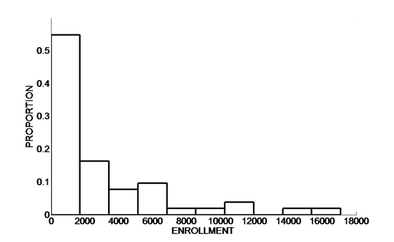
1. The median is equivalent to the __th percentile.

2. From the histogram, make a reasonable guess at the median enrollment. (Note: the vertical axis of this histogram is proportion instead of frequency. Try turning the proportions into percentages and percentile ranks, and you’d get a pretty good idea of where the median should be)

3. Based on the shape of the data, do you think the mean is larger or smaller than the median?

3. A 50-item mathematics test was given to the 150 students in five classes at Sunnyside School. Scores ranged from 16 to 50, with 93 of the students getting scores above 40. The mean score of these classes is 35. Is this distribution skewed? If so, to which direction? (Note: you can not answer this question with the help of R, since the original dataset is not available, but it would be helpful to try to draw a rough histogram of this distribution by hand)

4. For each of the three quantitative variables in the class survey data, find your own percentile rank, and explain what this number means.

5. Following is the answer to the question “how much did your last haircut cost” from a previous class. Use this data to compute 1) the range, 2) the five-number summary, 3) the IQR, 4) Is this distribution skewed or not? If skewed, to which direction?

15 0 0 20 10 100 40 25 10 160 50 15 30 50 4 25 0 75 150 30

6. The lore of the presidency talks about George Washington and Abraham Lincoln as natural leaders because their height commanded respect. Given that the average height of adult male in the US is 69.3 inches, it does seem that the presidents tend to be taller than average. Use the raw data in the following table to calculate the mean, the squared deviations, the variance, and the standard deviation of the height of presidents during the TV era either manually or using R.

President	Height	President	Height
Eisenhower	70.5	Reagan	73
Kennedy	72	Bush	74
Johnson	76	Clinton	74
Nixon	71.5	Bush	71.5
Ford	72	Obama	73
Carter	69.5	Trump	75