Chapter 5 Summarizing data

These notes accompany portions of Chapter 3 — Describing Data — of our textbook. The reading below is required, Whitlock and Schluter (2020) is not.

Motivating scenarios: You want to communicate simple summaries of your data or understand what people mean in their summaries.

Learning goals: By the end of this chapter, you should:

Be able to explain and interpret summaries of the location and spread of a dataset.
Recognize and use the mathematical formulae for these summaries.
Calculate these summaries in R.
Use a histogram to responsibly interpret a given numerical summary, and to evaluate which summary is most important for a given dataset (e.g. mean vs. median, or variance vs. interquartile range).

The other reading assignment for class is to watch the video about data summaries from Calling Bullshit (Bergstrom and West 2020), and this video from crash course on the shape of data.

5.1 Four things we want to describe

While there are many features of a dataset we may hope to describe, we mostly focus on four types of summaries:

The location of the data: e.g. mean, median, mode, etc…
The shape of the data: e.g. skew, number of modes, etc…
The spread of the data: e.g. range, variance, etc…
Associations between variables: e.g. correlation, covariance, etc…

Today we focus mainly on the spread and location of the data, as well as the shape of the data (because the meaning of other summaries depend on the shape of the data). We save summaries of associations between variables for later chapters.

When summarizing data, we are taking an estimate from a sample, and do not have a parameter from a population.

In stats we use Greek letters to describe parameter values, and the English alphabet to show estimates from our sample.

We usually call summaries from data sample means, sample variance etc. to remind everyone that these are estimates, not parameters. For some calculations (e.g. the variance) the equations to calculate the parameter from a population differ slightly from equations to estimate it from a sample, because otherwise estimates would be biased.

5.2 Data sets for today

We will continue to rely on the iris data set to work through these concepts.

5.3 Measures of location

FIGURE 5.1: Watch this video on Calling Bullshit on summarizing location (15 min and 05 sec).

We hear and say the word, “Average”, often. What do we mean when we say it? “Average” is an imprecise term for a middle or typical value. More precisely we talk about:

Mean (aka \(\overline{x}\)): The expected value. The weight of the data. We find this by adding up all values and dividing by the sample size. In math notation, this is \(\frac{\Sigma x_i}{n}\), where \(\Sigma\) means that we sum over the first \(i = 1\), second \(i = 2\) … up until the \(n^{th}\) observation of \(x\), \(x_n\). and divide by \(n\), where \(n\) is the size of our sample.
Median: The middle value. We find the median by lining up values from smallest to biggest and going half-way down.
Mode: The most common value in our data set.

Let’s explore this with the iris data.

To keep things simple, let’s focus on just the setosa, isolating it using the filter() function we encountered in Chapter 4. Let’s also arrange() these data from smallest to largest value to make it easiest to find the median.

setosa <- iris                           %>%
  janitor::clean_names()                 %>% # clean the names
  dplyr::tibble()                        %>% # make it a tibble (as opposed to a data frame)
  dplyr::filter(species == "setosa")     %>% # just get setosa
  dplyr::arrange(sepal_length)

DT::datatable(setosa, options = list(pageLength = 5, lengthMenu = c(5, 10, 20, 30)))

We can calculate the sample mean as \(\overline{x} = \frac{\Sigma{x_i}}{n}\) so,
\(\overline{x} = \frac{4.3 + 4.4 + 4.4 + 4.4 + 4.5 + 4.6 + \dots + 5.4 + 5.5 + 5.5 + 5.7 + 5.7 + 5.8}{50}\)
\(\overline{x} = \frac{250.3}{50}\)
\(\overline{x}= 5.006\)
We can calculate the sample median by going halfway down the table and take the value in the middle of our data.
- If we have an odd number of observations in our sample, this is the \(\frac{n+1}{2}^{th}\) value. For example, if we had 51 samples, the median is the \(\frac{51+1}{2}^{th} = \frac{52 }{2}^{nd} = 26^{th}\) sepal length in our sorted setosa data set. We can extract this value with the slice function as follows slice(setosa,26) %>% pull(sepal_length) = 5. Scroll through the data above to confirm.
- If we have an odd number of observations in our sample, this is the average of the \(\frac{n}{2}^{th}\) and \(\frac{n+1}{2}^{th}\) values. So in our actual \(n = 50\) dataset, the median is the average of the \(25^{th}\) and \(26^{th}\) sepal lengths in our sorted setosa data set, which equal 5 and 5, An the median of the dataset is the mean of these two values \(\frac{5+5}{2}=5\).

5.3.1 Getting summaries in R

As we saw in the previous chapter, the summarise() function in R reduces a data set to summaries that you ask it for. So, we have R find the mean and median with the mean() and median() functions and confirm the mean is correct by taking the sum and dividing by the sample size as follows. [please explore for yourself!]

Note, we can choose any name we want for these summarized columns - just make sure they follow best practices described in Chapter 2.

5.3.2 Getting summaries by group in R

Returning to our full iris data set, let’s say we wanted to get the sepal length mean for each species. As seen in the previous chapter, we can combine the group_by() and summarise() functions introduced above.

iris                                                   %>%
  group_by(Species)                                    %>%
  summarise(mean_sepal_length   = mean(Sepal.Length))

## # A tibble: 3 × 2
##   Species    mean_sepal_length
##   <fct>                  <dbl>
## 1 setosa                  5.01
## 2 versicolor              5.94
## 3 virginica               6.59

So, the Iris setosa sample has the shortest sepals, and the Iris virginica sample has the longest sepals. Later in the term, we consider how easily sampling error could generate such a difference between estimates from different samples.

If you type the code above, R will say something like summarise(…, .groups ="drop_last"). R is saying that it does not know which groups you want it to drop when you are summarizing (if you’re grouping by more than one thing, which we are not). To make this go away, type:

summarise(..., .groups = "drop_last") to drop the last thing in group_by(),
summarise(..., .groups = "drop") to drop all things in group_by(),
summarise(..., .groups = "keep") to drop no things in group_by(), or
summarise(..., .groups = "rowwise") to keep each row as its own group.

5.4 Summarizing shape of data

FIGURE 5.2: The shape of distributions from Crash Course Statistics.

Always look at the data before interpreting or presenting a quantitative summary. A simple histogram is best for one variable, while scatter plots are a good starting place for two continuous variables.

🤔WHY? 🤔 Because knowing the shape of our data is critical for making sense of any summaries.

5.4.1 Shape of data: Skewness

To help think about the shape of the data le’t look into the rivers dataset – a vector of lengths (in miles) of 141 “major” rivers in North America, as compiled by the US Geological Survey. Because ggplot requires tibbles, we first make a tibble which we call, river_tibble with one column, river_length, corresponding to river lengths,

river_tibble <- tibble(river_length = rivers) # Make the data into a tibble

ggplot(river_tibble, aes(x=river_length))+     # set up our aesthetics and data layers
  geom_histogram()                            # make a histogram (ignore code for added elaborations (labeling mean and median))

Histogram of river length dataset. The median is the <span style="color:red">dashed red line</span>, and the mean is shown by the <span style="color:blue">solid blue line</span>.

FIGURE 5.3: Histogram of river length dataset. The median is the dashed red line, and the mean is shown by the solid blue line.

We notice two related things about Figure 5.3:
1. There are a numerous extremely large values.
2. The median is substantially less than the mean.

We call data like that in Figure 5.3 Right skewed, while data with an excess of extremely small values, and with a median substantially greater than the mean are Left skewed.

In Figure 5.4, we show example density plots of left-skewed, unskewed, and right-skewed data.

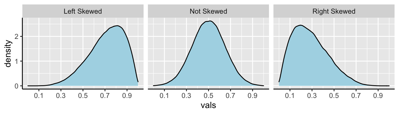
FIGURE 5.4: Examples of skew.

For skewed data sets, the median is often a more relevant description of the data set than the mean, because it better describes a typical data point.*

5.4.2 Shape of data: Unimodal, bimodal, trimodal

The number of “peaks” or “modes” in the data is another important descriptor of its shape, and can reveal important things about the data. If Edgar Anderson came to us with his iris dataset (before he collected the Iris versicolor data), and showed us a plot of sepal lengths, without telling us which species each data point came from, we would make the plots below.

no_versicolor <- dplyr::filter(iris, Species != "versicolor") 

hist_no_versicolor <- ggplot(no_versicolor, aes(x = Sepal.Length))+
  geom_histogram(color = "white")

dense_no_versicolor <- ggplot(no_versicolor, aes(x = Sepal.Length))+
  geom_density(fill = "orange")

library(patchwork) # You DONT need to know this! But it allows us to combin plots with a + sign
hist_no_versicolor + dense_no_versicolor

FIGURE 5.5: Example of bimodal data

Figure 5.5 shows two “peaks” – one near 5.0, and one near 6.6 – thus these data are bimodal. Bimodal data suggests (but does not always mean) that we have sampled from two populations.

As revealed in Figure 5.6 each peak is associated with a different species, and data are unimodal (have one peak) within species.

hist_no_versicolor <- ggplot(no_versicolor, aes(x = Sepal.Length, fill = Species))+   geom_histogram(color = "white")
dense_no_versicolor <- ggplot(no_versicolor, aes(x = Sepal.Length, fill = Species))+ geom_density(alpha = .5)

library(cowplot) # You DONT need to know this! It's a fancier way to combine polts allowing us to combine our legend
plot_grid(hist_no_versicolor+theme(legend.position = "none"), 
          dense_no_versicolor+theme(legend.position = "none"), 
          get_legend(hist_no_versicolor), 
          ncol =3, 
          rel_widths = c(2,2,1))

FIGURE 5.6: Example of bimodal data

Figure 5.7 reminds us that there can be three modes or more!

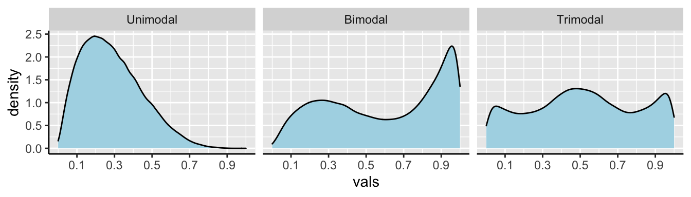
FIGURE 5.7: Examples of unimodal, bimodal, and trimodal data.

Although multimodal data suggest (but do not guarantee) that samples originate from multiple populations, data from multiple populations can also looks unimodal when those distributions blur into each other. For example, combining sepal lengths from all three iris species results in a unimodal distribution (Fig 5.8).

dense_iris_density <- ggplot(iris, aes(x = Sepal.Length))+ geom_density(fill="orange",alpha = .5)
dense_iris_density_by_sp <- ggplot(iris, aes(x = Sepal.Length, fill = Species))+ geom_density(alpha = .5)

plot_grid(dense_iris_density +theme(legend.position = "none"), 
          dense_iris_density_by_sp +theme(legend.position = "none"), 
          get_legend(dense_iris_density_by_sp), ncol =3, rel_widths = c(2,2,1))

FIGURE 5.8: Data from multiple (statistical) populations can appear to be unimodal

5.5 Measures of width

Variability (aka width of the data) is not noise that gets in the way of describing the location. Rather, the variability in a population is itself an important biological parameter which we estimate from a sample. For example, the key component of evolutionary change is the extent of genetic variability, not the mean value in a population.

Common measurements of width are the

Range: The difference between the largest and smallest value in a data set.
Interquartile range (IQR): The difference between the \(3^{rd}\) and \(1^{st}\) quartiles.
Variance: The average squared difference between a data point and the sample mean.
Standard deviation: The square root of the variance.
Coefficient of variation: A unitless summary of the standard deviation facilitating the comparison of variances between variables with different means.

5.5.1 Measures of width: Boxplots, Ranges and Interquartile range (IQR)

We call the range and the interquartile range nonparametric because we can’t write down a simple equation to get them, but rather we describe a simple algorithm to find them (sort, then take the difference between things).

Let’s use a boxplot to illustrate these summaries.

ggplot(iris , aes(x=Species, y= Sepal.Length, color = Species))+
  geom_boxplot() +
  labs(title = "Boxplot of Iris sepal lengths") +
  theme(legend.position = "none")  +
  facet_wrap(~Species, scales = "free_x")

Boxplot of Iris sepal length. Boxplots display the four quartiles of our data (noted on the center versicolor facet). 75% of data points fall within the *box*, and the interquartile range is the difference between the top and bottom of the box. Extreme data points (aka outliers) are shown with a point, as seen in the *virginica* facet.

FIGURE 5.9: Boxplot of Iris sepal length. Boxplots display the four quartiles of our data (noted on the center versicolor facet). 75% of data points fall within the box, and the interquartile range is the difference between the top and bottom of the box. Extreme data points (aka outliers) are shown with a point, as seen in the virginica facet.

We calculate the range by subtracting min from max (as noted in Fig. 5.9). But because this value increases with the sample size, it’s not super meaningful, and it is often given to provide an informal description of the width, rather than a serious statistic. I note that sometimes people use range to mean “what is the largest and smallest value?” rather than the difference between theme (in fact that’s what the range() function in R does).
We calculate the interquartile range (IQR) by subtracting Q1 from Q3 (as shown in Fig. 5.9). The IQR is less dependent on sample size than the range, and is therefore a less biased measure of the width of the data.

5.5.1.1 Calculating the range and IQR in R.

Staying with the iris data set, let’s see how we can calculate these summaries in R. As I showed with the mean, I’ll first work through example codes that shows all the steps and helps us understand what we are calculating, before showing R shortcuts.

To calculate the range, we need to know the minimum and maximum values, which we find with the min() and max().

To calculate the IQR, we find the \(25^{th}\) and \(75^{th}\) percentiles (aka Q1 and Q3), by setting the probs argument in the quantile() function equal to 0.25 and 0.75, respectively.

iris %>% 
  group_by(Species) %>%
  summarise(length_max   = max(Sepal.Length),
            length_min   = min(Sepal.Length),
            length_range = length_max - length_min,
            length_q3    = quantile(Sepal.Length, probs = c(.75)),
            length_q1    = quantile(Sepal.Length, probs = c(.25)),
            length_iqr   = length_q3 - length_q1 ) %>%
  dplyr::select(length_iqr, length_range)

## # A tibble: 3 × 2
##   length_iqr length_range
##        <dbl>        <dbl>
## 1      0.400          1.5
## 2      0.7            2.1
## 3      0.675          3

Or we can get use R’s built in R functions

Get the interquartile range with the built-in IQR() function, and
Get th difference between largest and smallest values by combining the range() and diff() functions.

iris %>% 
  group_by(Species) %>%
  summarise(sepal_length_IQR   = IQR(Sepal.Length) ,
            sepal_length_range = diff(range(Sepal.Length) ))

## # A tibble: 3 × 3
##   Species    sepal_length_IQR sepal_length_range
##   <fct>                 <dbl>              <dbl>
## 1 setosa                0.400                1.5
## 2 versicolor            0.7                  2.1
## 3 virginica             0.675                3

5.5.2 Measures of width: Variance, Standard Deviation, and coefficient of variation.

The variance, standard deviation, and coefficient of variation all communicate how far individual observations are expected to deviate from the mean. However, because (by definition) the differences between all observations and the mean sum to zero (\(\Sigma x_i = 0\)), these summaries work from the squared difference between observations and the mean.

To work through these ideas and calculations, let’s return to the Iris setosa sepal length data sorted from shortest to longest. As a reminder, the sample mean was 5.006. Before any calculations, lets make a simple plot to help investigate these summaries:

Visualizing variability in the Iris setosa style lengths. **A)** The red dots show the sepal length of each *Iris setosa* plant , and the solid black lines show the difference between these values and the mean (dotted line). **B)** Every sepal length is shown on the x-axis. The y-axis shows the squared difference between each observation and the sample mean. The solid black line highlights the extent of these values.

FIGURE 5.10: Visualizing variability in the Iris setosa style lengths. A) The red dots show the sepal length of each Iris setosa plant , and the solid black lines show the difference between these values and the mean (dotted line). B) Every sepal length is shown on the x-axis. The y-axis shows the squared difference between each observation and the sample mean. The solid black line highlights the extent of these values.

Calculating the sample variance:

The sample variance, which we call \(s^2\) is the sum of squared differences of each observation from the mean, divided by the sample size minus one. We call the numerator ‘sums of squares x’, or \(SS_x\).

\[s^2=\frac{SS_x}{n-1}=\frac{\Sigma(x_i-\overline{x})^2}{n-1}\].

Here’s how I like to think the steps:

Getting a measure of the individual differences from the mean, then
Squaring those diffs to get all the values positive,
Adding all those up, then dividing them to get something close to the mean of the differences.
Instead of dividing by N though, we use N-1 to adjust for sample sizes (as we get larger numbers, the -1 gets diminishingly less consequential).

We know that this dataset contains 50 observations and so \(n-1 = 50-1=49\), so let’s work towards calculating the Sums of Squares x, \(SS_x\).

Figure 5.10A highlights each value of \(x_i - \overline{x}\) as the length of each line. Figure 5.10B plots the square of these values, \((x_i-\overline{x})^2\) on the y, again highlighting these squared deviations with a line. So to find \(SS_x\), we

Take each observation,
Subtract away the mean,
Square this value for each observation.
Sum across all observations.

For the setosa data set it looks like this \(SS_x = (4.3 - 5.006)^2 + (4.4 - 5.006)^2 + (4.4 - 5.006)^2 + (4.4 - 5.006)^2 + (4.5 - 5.006)^2 + (4.6 - 5.006)^2 \dots\) with those dots meaning that we kept doing this for all fifty observations.

Doing this, we find \(SS_x = 6.0882\), and we find the sample variance as \(SS_x / (n-1) = 6.0882/49 = 0.124249\).

Calculating the sample standard deviation:

The **sample standard deviation*, which we call \(s\), is simply the square root of the variance. So \(s = \sqrt{s^2} = \sqrt{\frac{SS_x}{n-1}}=\sqrt{\frac{\Sigma(x_i-\overline{x})^2}{n-1}}\). So for the example above the sample standard deviation, \(s\) equals \(\sqrt{0.124} = 0.352\).

🤔 You may ask yourself 🤔 when should you report / use the standard deviation vs the variance? Because they are super simple mathematical transformations of one another, it is usually up to you, just make sure you communicate clearly.

🤔 You may ask yourself 🤔 why teach/learn both the standard deviation and the variance? We teach because both are presented in the literature, and because sometimes one these values or the other naturally fits in a nice equation.

Calculating the sample coefficient of variation

The sample coefficient of variation standardizes the sample variance by the sample mean. So the sample coefficient of variation equals the sample standard deviation divided by the sample mean, multiplied by 100, \(CV = 100 \times \frac{s}{\overline{x}}\). So for the example above the sample coefficient of variation equals \(100 \times \frac{0.352}{5.006} = 0.07\%\).

The standard deviation often gets bigger as the mean increase. Take, for example, measurements of weight for ten individuals calculate in pounds or stones. Because there are 14 pounds in a stone, the variance for the same measurements on the same individuals will be fourteen times bigger for measurements in pounds relative to stone. Dividing by the mean removes this effect. Because this standardization results in a unitless measure, we can then meaningfully ask questions like “What is more variable, human weight or the rate or dolphin swim speed.”

🤔You may ask yourself 🤔 when should you report the standard deviation vs the coefficient of variation?

When we are sticking to our study, it is nice to present the standard deviation, because we do not need to do any conversion to make sense of this number.
When comparing studies with different units or measurements, consider the coefficient of variation.

Calculating the variance, standard deviation, and coefficient of variation in R.

Calculating the variance, standard deviation, and coefficient of variation with math in R.

We can calculate these summaries of variability with learning very little new R! Let’s work through this step by step:

# Step one, find the mean and the squared deviation  
iris_var <- iris                           %>% 
     dplyr::select(Species, Sepal.Length)  %>%                           # let's just show the sepal lengths         
     group_by(Species)                     %>%                           # calculate separate means for each species
     mutate(deviation_sepal_length = Sepal.Length - mean(Sepal.Length),  # find each observation's deviation from the species' mean
            sqrdev_sepal_length    = (deviation_sepal_length)^2)         # find each observation's squared deviation from the species' mean

So, now that we have the squared deviations, we can calculate all of our summaries of interest.

iris_var  %>%
    dplyr::summarise(variance_sepal_length = sum(sqrdev_sepal_length)  / (n()-1), # find the variance by summing the squared deviations and dividing by n-1
                     stddev_sepal_length   = sqrt(variance_sepal_length),         # find the standard deviation as the square root of the variance
                     coefvar_sepal_length  = 100 * stddev_sepal_length / mean(Sepal.Length )) #make variability comparable across species by turning the standard deviation into a coefficient of variation

## # A tibble: 3 × 4
##   Species    variance_sepal_length stddev_sepal_length
##   <fct>                      <dbl>               <dbl>
## 1 setosa                     0.124               0.352
## 2 versicolor                 0.266               0.516
## 3 virginica                  0.404               0.636
## # … with 1 more variable: coefvar_sepal_length <dbl>

Calculating variance and related measures with built in R functions.

The code above shows us how to calculate these values with math, but as we saw with the mean() function, R often has a built-in function to do common statistical procedures, so there’s no sense in writing the code above for a serious analysis. We can use the var() and sd() functions to calculate these summaries more directly.

iris                                                              %>%         # the data
  group_by(Species)                                               %>%         # calculate separately for each species
  summarise(mean_sepal_length    = mean(Sepal.Length),                        # mean
            var_sepal_length     =  var(Sepal.Length),                        # variance
            sd_sepal_length      =   sd(Sepal.Length),                        # standard deviation
            coefvar_sepal_length = 100 * sd_sepal_length / mean_sepal_length) # coefficient of variation

## # A tibble: 3 × 5
##   Species    mean_sepal_length var_sepal_length
##   <fct>                  <dbl>            <dbl>
## 1 setosa                  5.01            0.124
## 2 versicolor              5.94            0.266
## 3 virginica               6.59            0.404
## # … with 2 more variables: sd_sepal_length <dbl>,
## #   coefvar_sepal_length <dbl>

5.6 Parameters and estimates

Above we discussed estimates of the mean (\(\overline{x} = \frac{\Sigma{x_i}}{n}\)), variance (\(s^2 = \frac{SS_x}{n-1}\)), and standard deviation (\(s = \sqrt{\frac{SS_x}{n-1}}\)). We focus on estimates because we usually have data from a sample and want to learn about a parameter from a sample.

If we had an actual population (or, more plausibly, worked on theory assuming a parameter was known), we use Greek symbols and have slightly difference calculations.

The population mean \(\mu = \frac{\Sigma{x_i}}{N}\).
The population variance = \(\sigma^2 = \frac{SS_x}{N}\).
The population standard deviation \(\sigma = \sqrt{\sigma^2}\).

Where \(N\) is the population size.

🤔 ?Why? 🤔 do we divide the sum of squares by \(n-1\) to calculate the sample variance, and but divide it by \(N\) to calculate the population variance?

Estimate of the variance are biased to be smaller than they actually are if we divide by n (because samples go into estimating the mean too). Dividing by n-1 removes this bias. But if you have a population you are not estimating the mean, you are calculating it, so you divide by N. In any case, this does not matter too much as sample sizes get large.

5.7 Rounding and number of digits, etc…

How many digits should you present when presenting summaries? The answer is: be reasonable.

Consider how much precision you would you care about, and how precise your estimate is. If i get on a scale and it says I weigh 207.12980423544 pounds. I would probably say 207 or 207.1 because scales are generally not accurate to that level or precision.

To actually get R value’s from a tibble we have to pull() out the vector and round() as we see fit. If we don’t pull(), we have to trust that tidyverse made a smart, biologically informed choice of digits – which seems unlikely. If we do not round, R gives us soooo many digits beyond what could possibly be measured and/or matter.

# Example pulling and rounding estimates
# not rounding
summarise(setosa, mean_sepal_length = mean(sepal_length)) %>%  # get the mean
  pull(mean_sepal_length)                                      # pull it out of the tibble

## [1] 5.006

# rounding to two digits
summarise(setosa, mean_sepal_length = mean(sepal_length)) %>%  # get the mean
  pull(mean_sepal_length)                                 %>%  # pull it out of the tibble
  round(digits =2)                                             # round to two digits

## [1] 5.01

5.8 Summarizing data quiz

Summarizing data: Definitions, Notation, Equations, and Useful functions

Summarizing data: Definitions, Notation, and Equations

Location of data: The central tendency of the data.
Width of data: Variability of the data.

Summarizing location
Mean: The weight of the data, which we find by adding up all values and dividing by the sample size.
- Sample mean \(\overline{x} = \frac{\Sigma x}{n}\).
- Population mean \(\mu = \frac{\Sigma x}{N}\).
Median: The middle value. We find the median by lining up values from smallest to biggest and going half-way down.
Mode: The most common value in a dataset.

Summarizing width
Range: The difference between the largest and smallest value.
Interquartile range (IQR): The difference between the third and first quartile.
Sum of squares: The sum of the squared difference between each value and its expected value. Here \(SS_x = \Sigma(x_i - \overline{x})^2\).
Variance The average squared difference between an observations and the mean for that variable.
- Sample variance: \(s^2 = \frac{SS_x}{n-1}\)
- Population variance: \(\sigma^2 = \frac{SS_x}{N}\)
Standard deviation: The sqaure root of the variance.
- Sample standard deviation: \(s=\sqrt{s^2}\).
- Population standard deviation: \(\sigma=\sqrt{\sigma^2}\).
Coefficient of variation: A unitless summary of the standard deviation facilitating the comparison of variances between variables with different means. \(CV = 100 \times \frac{s}{\overline{x}}\).

Here are the functions we came across in this chapter that help us summarize data.

If your vector has any missing data (or anything else R seen as NA, R will return NA by default when we ask for summaries like the mean, media, variance, etc… This is because R does not know what these missing values are.

To override this and get summaries excluding NA values add the na.rm = TRUE, e.g. summarise(mean(x,na.rm = TRUE)).

General functions
group_by(): Conduct operations separately by values of a column (or columns).
summarise():Reduces our data from the many observations for each variable to just the summaries we ask for. Summaries will be one row long if we have not group_by() anything, or the number of groups if we have.
sum(): Adding up all values in a vector.
diff(): Subtract sequential entries in a vector.
sqrt(): Find the square root of all entries in a vector.
unique(): Reduce a vector to only its unique values.
pull(): Extract a column from a tibble as a vector.
round(): Round values in a vector to the specified number of digits.

Summarizing location
n(): The size of a sample.
mean(): The mean of a variable in our sample.
median(): The median of a variable in our sample.

Summarizing width
max(): The largest value in a vector.
min(): The smallest value in a vector.
range(): Find the smallest and larges values in a vector. Combine with diff() to find the difference between the largest and smallest value…
quantile(): Find values in a give quantile. Use diff(quantile(... , probs = c(0.25, 0.75))) to find the interquartile range.
IQR(): Find the difference between the third and first quartile (aka the interquartile range).
var(): Find the sample variance of vector.
sd(): Find the sample standard deviation of vector.

References

Bergstrom, Carl T, and Jevin D West. 2020. Calling Bullshit: The Art of Skepticism in a Data-Driven World. Random House.

Whitlock, Michael C, and Dolph Schluter. 2020. The Analysis of Biological Data. Third Edition.