Chapter 27 Designing scientific studies
Motivating scenarios: We want to plan a study or we are critically evaluating claims made by others.
Learning goals: By the end of this chapter you should be able to
- Name four potential reasons two variables two variables can be correlated.
- Explain why (good) experiments allow us to learn about causation.
- Explain why a experiment does might not necessarily imply causation in the world.
- Consider if/how we can infer causation without an experiment.
- Recognize the paths researchers can take to minimize bias in their research.
- Describe the placebo effect and why and the limitations of causal claims from experiments.
- Recognize the best practices researchers can take to minimize sampling error.
- Describe the concept of statistical power and how we can use simulation and/or math to learn about the power of a study.
27.1 Review / Set up
To consult the statistician after an experiment is finished is often merely to ask him to conduct a post mortem examination. He can perhaps say what the experiment died of.
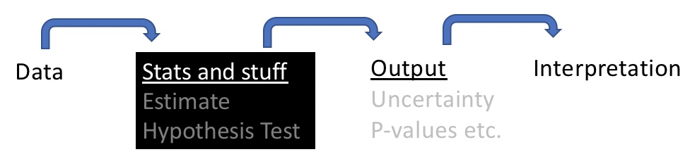
In Chapter 1 we introduced the major goals of statistics. In order of importance, they are:
- Inferring causation – If two variables are actually associated, (how) can we know if one caused the other?
- Estimation (with uncertainty) – How can we responsibly describe aspects of the world with our limited view of it from a finite sample.
- Hypothesis testing – Can a pattern in a sample be reasonably explained by invoking the vagaries of sampling from a boring, “null” sampling distribution, or is this an unlikely explanation.
So far, we’ve mainly dealt with cases in which someone else did an experiment and looked at their study design and raw data to meet these goals.
In this chapter, we are considering how we would design a study. There are two very good reasons for this.
- Many of you will end up conducting some form of scientific study in your life.
- Even if you never do a scientific study, considering how to design a good study helps us understand both the reasoning behind and shortcomings of scientific studies / claims.
27.2 Challenges in inferring causation
We have spent the past few weeks digging into the details of statistical methods, counting up our sums of squares, and finding how weird it would often a sample from the null sampling distribution would be as or more extreme than our estimate. This is a noble goal – we know that sample estimates can differ from population parameters due to chance, and we want to be skeptical so as not to be lied to by data.
However, as we focus on significance and uncertainty we can sometimes lose the bigger picture. That is, we need to focus on what we can and cannot conclude from a study even if it showed a significant result. Another way to say this is that we have delved into the black box in some depth, but have spent a lot less effort thinking about the interpretation of the results. We need to fix this because all of our statistical wizardry and talents are wasted if we do not critically consider the e implications of a study. We will begin thinking about this formally here and continue in future chapters.
When thinking about the implications of a study, we need to consider the goals and message of the work.
- If the goal is simply to make a prediction, we need not worry about causation, instead we worry about sampling bias and sampling error etc etc..
- However, many people do research to make causal claims. For example, if I’m considering exercising regularly to increase my lifespan, I don’t want to know if people who exercise live longer – they could be living longer because of a part of their healthy diet. Rather, I want to know if taking up exercise will likely on average increase my lifespan.
Watch video (27.1) for a discussion of correlation and causation.
FIGURE 27.1: Watch this 8 minute video on correlation and causation from Calling Bullshit.
27.2.1 Correlation does not necessarily imply causation
What does this mean? It’s not just about \(r\) – rather, it’s saying that statistical associations between two variables, A and B, do not mean that e.g. B caused A. That if lm(A~B) %>% anova() yields p-value < 0.05, we cannot necessarily conclude that B caused A (A could cause B, or both could be caused by C, or this could be a false positive, etc…, Figure 27.2).
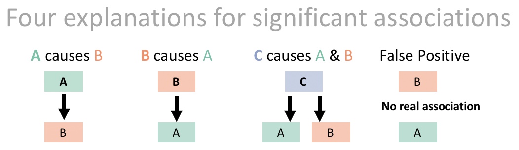
FIGURE 27.2: Possible causal relationships underlying significant associations. In this example, we would call C a *confounding variable**.
Remember a p-value just tells us how incompatible the data are with the null model, not what’s responsible for this incompatibility. Watch the brief video below for a fun example 27.3. Note that at the end of the video, she discusses the problem of
FIGURE 27.3: Watch from 8:02 to 10:26 of the Correlation Doesnt Equal Causation video from Crash Course Statistics.
27.3 One weird trick to infer causation
Experiments offer us a potential way to learn about causation. In a well-executed experiment, we randomly assign individuals to treatment groups, to prevent an association between treatments and any confounding variables. Watch the video below (27.4) to hear a nice explanation of experiments and their limitations.
FIGURE 27.4: Watch the first 4 minutes of this video on manipulative experiments from Crash course on statistics. We will watch the rest of this video as we move through these concepts.
27.3.1 When experiments are not enough
27.3.1.1 False negatives and power
Absence of evidence is not evidence of absence.
Say we did an experiment and failed to reject the null. Remember that does not mean that the null is true. There still could be a causal relationship. We Revisit this in our discussion of power.
27.3.1.2 Cause in experiment \(\neq\) cause in the real world
Experiments are amazing, and are among our best ways to demonstrate causation. Still, we have to be careful in interpreting results from a controlled experiment.
A causal relationship in an experiment does not imply a causal relationship in the real world, even for a true positive with a well-executed experiment. Here are some things to consider:
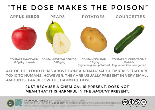
Treatment severity Remember the toxicology adage, “The dose makes the poison.” When an experimental treatment has an effect we should step back for a minute, and think about whether the level of exposure in the experimental treatment was comparable to what we see in our observational study. If not, it is possible that the treatment was causal in the experiment, but may not be relevant at real world doses.
Comparable effect sizes Say an experimental treatment had an effect – say in an experimental study we find that studying an extra hour for an exam increases test scores by 1.5%. This would show that studying can increase test scores, but would not explain a 15% difference in test scores for students who studies, an average, an hour longer than those in another group.
Interactions Most experiments happen in a controlled setting in a lab. Most published research studies WEIRD (Western, educated, industrialized, rich and democratic) populations etc. In Chapter 24 we addressed the idea of interactions. So, we might worry if an experimental study is used as causative evidence for a claim concerning a very different context. Similarly, an absence of a causal relationship in an experiment might be misleading if an interaction between the treatment and some other variable which was not studies was the true cause.

- Multiple causes In the real world, more than one thing can another. Showing that A causes B in an experiment does not mean that C does not cause B.
27.4 Minimizing bias in study designs
Experiments allow us to infer causation because they remove the association between the variable we care about and any confounding variables.
So, we better be sure that we don’t introduce covariates as we do our experiment. For these reasons, the best experiments include
- Realistic controls
- Hiding the true treatment from and experimenters
27.4.1 Potential Biases in Experiments
Time heals Whenever I feel terribly sick, I call the doctor, and usually get an appointment the following week. Most of the time I get better before seeing the doctor. I therefore joke that the best way for me to get better is to schedule a doctor appointment. Now let’s think about this – obviously calling the Dr. didn’t heal me. Rather I called the Dr. when I felt my worst, and got better with time. This is because we tend to get better.
Regression to the mean A related concept, known as “Regression to the Mean” is the idea that the most extreme observations in a study are biased estimates of the true parameter values. That’s because being exceptional requires both an expectation of being exceptional (extreme \(\widehat{Y_i}\)) AND a high residual in that same direction (i.e. large positive and large negative residuals for exceptionally large and small values, respectively.
Experimental artifacts The experimental manipulation itself, rather than the treatment we care about could be causing the experimental result. Says we hypothesize that birds are attracted to red, so we glue red feathers onto some birds and see that that increases their mating success. We want to make sure that it is the red color, not the glue or added feathers that drives this elevated attractiveness.
Known treatments are a special kind of experimental artifact. Knowledge of the treatment by either the experimental subject or the experimenter, can introduce a bias. For example, people who think they have gotten treated might prime themselves for improvement. Processes like these are known as a placebo effect (listen to the 7 minute clip from radiolab, below for examples of the placebo and how it may work). Or, if the researchers know the treatment they may subconsciously bias their measurements or the way the treat their subjects.
27.4.2 Eliminating Bias in Experiments
We can minimize these biases by
Introducing effective controls It’s usually a good idea to have a “do nothing” treatment as a control, but this is not enough. We should also include a “sham treatment” or “placebo” is identical to the treatment in every way but the treatment itself. Taking our bird feathers example, we would introduce a treatment in which we glued blue feathers, and maybe ne where we glued on black feathers, to ensure the color red was responsible for the elevated attractiveness observed in our study.
“Blinding” If possible, we should do all we can to ensure that neither te experimenter nor the subjut knows which treatment they received.
Watch the video below from Crash Course in Statistics for a discussion of controls, placebos and blinding in experimental design.
FIGURE 27.5: Watch from 4:48 to 7:02 of this video on controls, placebos, and blinding from Crash course on statistics. We will watch the rest of this video as we move through these concepts.
27.5 Inferring causation when we can’t do experiments
Experiments are our best way to learn about causation, but we can’t always do experiments. Sometimes they are unethical, other times they are cost-prohibitive, or simply impossible. Do we have any hope of inferring causation in these cases?
The short answer is – sometimes, if we’re lucky. We return to this idea in discussions of causal inference in Chapter 33.
One good way to make causal claims from observational studies is to find matches, or “natural experiments” in which the variable we cared about changed in one set of cases, but did not in paired cases that are similar in every way except this change.
If we cannot make a rigorous causal claim it is best not to pretend we can. Rather, we should honestly describe what we can and cannot infer from our data.
FIGURE 27.6: Watch from 10:18 to 11:12 of this video on manipulative experiments from Crash course on statistics. We will watch the rest of this video as we move through these concepts.
27.6 Minimizing sampling error
Sampling bias isn’t our only consideration when planning a study, we would also like to increase our precision by decreasing sampling error.
Recall that sampling error is the chance deviation between an estimate and its true parameter which arises because of the process of sampling, and that we can summarize this as the standard deviation of the sampling distribution (aka the standard error). The standard error is something like the standard deviation divided by the square root of the sample size, so we can minimize sampling error by:
- Increasing the sample size or
- Decreasing the standard deviation
27.6.1 Increasing the sample size decreases sampling error.
Well of course! We learned this as the law of large numbers. Just be sure that our samples are independent… eg avoid pseudoreplication.
27.6.2 How to decrease the standard deviation.
We want to minimize, the standard deviation, but how? Well, we only have so much control of this because some variability is natural. Still there are things we can do
- More precise measurements More careful counting, fancier machines etc etc can provide more accurate measurements for each individual in our sample and eliminating this extraneous variability should decrease variability in our sample.

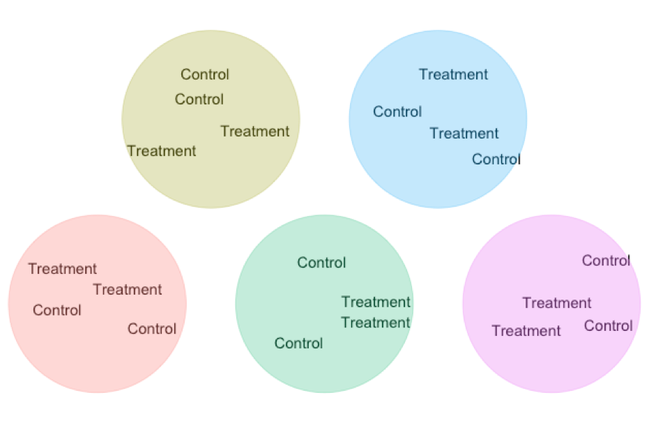
- Balanced design Balance refers to the similarity in sample sizes for each treatment. Recall that \(SE_{\overline{Y_1}-\overline{Y}_2} = \sqrt{s_p^2(\frac{1}{n_1}+\frac{1}{n_2})}\). So, for a fixed total sample size, more balanced experiments decrease uncertainty mean differences between treatments.
- Matching / Blocking A standard experimental design is two randomize who gets the treatment and wo get the control. But we can do even better than that!!! In Chapter 18, we saw that a paired t-test gets extra power by comparing natural pairs who are alike in many ways except the treatment. This design decreases variability in our estimated difference because in each pairs we minimize extraneous variation unrelated to treatment. We can scale that principle up to larger studies ANOVAs etc….
FIGURE 27.7: Watch from 8:57 to 10:06 of this video on manipulative experiments from Crash course on statistics. We will watch the rest of this video as we move through these concepts.
27.7 Planning for power and precision
We could maximize our power and precision by having an infinitely large sample, but this is obviously silly. We’d be wasting a bunch of time and resources over-doing one study and will miss out on so many others. So, how do we plan a study that is big enough to satisfy our goals, without overdoing it?
We need to think about the effect size we care about and the likely natural variability
- How precise of an estimate do we need for our biological story? In some cases, small difference mean a lot, in other cases, ballpark estimates are good enough. It’s your job as the researcher to know what is needed for your question.
- What effect size is worth knowing about? The null hypothesis is basically always false. With an infinite sample size, we’d probably always reject it. But in many of these cases, the true population parameter is so close to zero, that the null hypothesis might as well be true. Again, it’s your job as a researcher to consider what size of an effect you would like to be able to see.
- How much variability do we expect between measurements. Again, your biological knowledge is required here (or you could consider difference relative to variability when considering precision and effect size of interest)
27.7.1 Estimating an appropriate sample size.
We use power analyses to plan appropriate sample sizes for a study. A power analysis basically finds the sample size necessary so that the sampling distribution of your experiment has
- Some specified power to differentiate between the null model and the smallest effect size that you would like to be able to identify and/or
- Probability of being as or more precise than you want.
The traditional specified power researchers shot for is 80%, but in my opinion that is quite low and aiming for 90% power seems more reasonable.
The are numerous mathematical rules of thumb for power analyses, as well as online plugins e.g. this one from UBC and R packages (pwr is most popular)
27.7.2 Simulating to estimate power and precision
Here I focus on one way we can estimate power and precision – we can simulate!!! There is a bit on new R in here, including writing functions. Enjoy if you like, skim if you don’t care. I also note that there are more efficient ways to code this in R. I ca provide examples if there is enough demand.
Let’s first write our own function to
- Simulate data from two populations with a true mean difference of
x(the minimal value we care about) and a standard deviation of s from a normal distribution.
- Run a two sample t.test.
simTest <- function(n1, n2, x, s){
  sim_id  <- runif(1) # picka random id, in case you want it
  sim_dat <- tibble(treatment   = rep(c("a","b"), times = c(n1, n2)),
                    exected_val = case_when(treatment == "a" ~ 0,
                                            treatment == "b" ~ x)) %>%
    mutate(sim_val     = rnorm(n = n(),mean = exected_val, sd = s))
  tidy_sim_lm <- lm(sim_val ~ treatment, data = sim_dat) %>%
    broom::tidy() %>%
    mutate(n1 = n1, n2 = n2, x = x, s = s, sim_id = sim_id)
  return(tidy_sim_lm)
}
We can see the outcome of one random experiment, with a sd of 2, and a difference of interest equal to one, and a sample size of twenty for each treatment.
one_sim <- simTest(n1 = 20, n2 = 20, x = 1, s = 2)
one_sim                                                                                                                                                               %>% mutate_if(is.numeric,round,digits = 4) %>%DT::datatable( options = list( scrollX='400px'))
We probably want to filter for just treatmentb, because we don’t care about the intercept
filter(one_sim, term == "treatmentb")## # A tibble: 1 × 10
## term estimate std.error statistic p.value n1
## <chr> <dbl> <dbl> <dbl> <dbl> <dbl>
## 1 treatmentb 2.55 0.614 4.15 1.79e-4 20
## # … with 4 more variables: n2 <dbl>, x <dbl>, s <dbl>,
## # sim_id <dbl>We can replicate this many times
n_reps <- 500
many_sims <- replicate(simTest(n1 = 20, n2 = 20, x = 1, s = 2), n = n_reps, simplify = FALSE) %>%
  bind_rows() %>% # shoving output togther
  filter(term == "treatmentb")

many_sims                                                                                                                                                      %>%                                               mutate_if(is.numeric,round,digits = 4) %>%DT::datatable( options = list(pageLength = 5, lengthMenu = c(5, 25, 50), scrollX='400px'))
We can summarize this output to look at our power and the standard deviation, and upport and lower 2.5% quantiles to estimate our precision
many_sims %>%
  summarise(power        = mean(p.value < 0.05),
            mean_est     = mean(estimate),
            sd_est       = sd(estimate),
            lower_95_est = quantile(estimate, prob = 0.025),
            upper_95_est = quantile(estimate, prob = 0.975))
## # A tibble: 1 × 5
## power mean_est sd_est lower_95_est upper_95_est
## <dbl> <dbl> <dbl> <dbl> <dbl>
## 1 0.312 0.987 0.606 -0.208 2.19We can turn this last bit into a function and try it for a bunch of sample sizes
## # A tibble: 4 × 6
##       n power mean_est sd_est lower_95_est upper_95_est
##   <dbl> <dbl>    <dbl>  <dbl>        <dbl>        <dbl>
## 1    10 0.188    0.989  0.898       -0.648         2.76
## 2    20 0.338    0.985  0.631       -0.267         2.13
## 3    50 0.726    1.03   0.403        0.209         1.80
## 4   100 0.944    1.01   0.281        0.420         1.54