Chapter 35 Collecting and storing data
Motivating scenario: We start at the beginning of a study – how do we set up a good way to keep track of data that will allow us to focus on understanding and analyzing our data, not reorganizing and rearranging it?
Learning goals: By the end of this chapter you should be able to
- Describe best principles for collecting, storing, and maintaining data.
- Explain why these are good ideas.
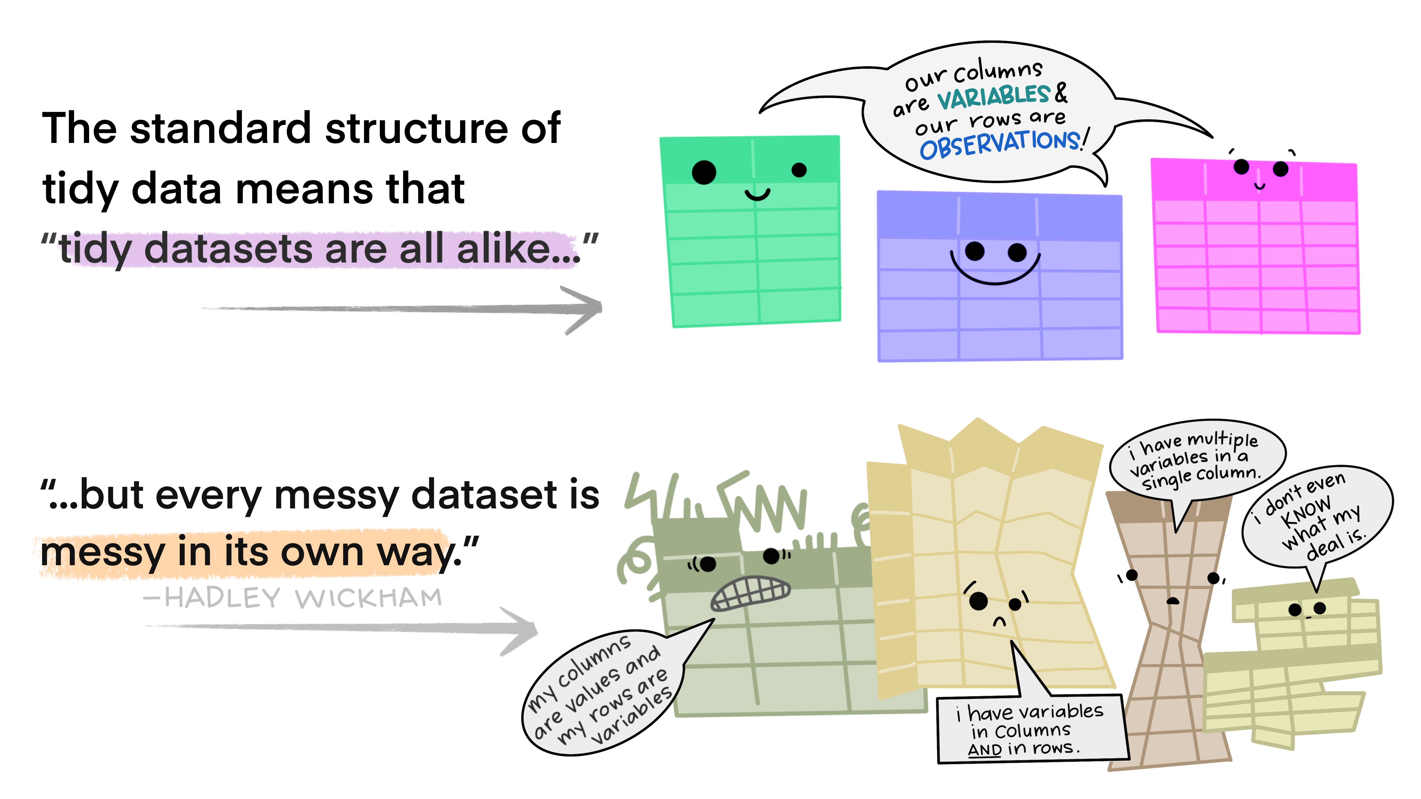
- Differentiate between tidy and messy data.
- Load data into R using a project
(1) Data Organization in Spreadsheets (Broman and Woo 2018).
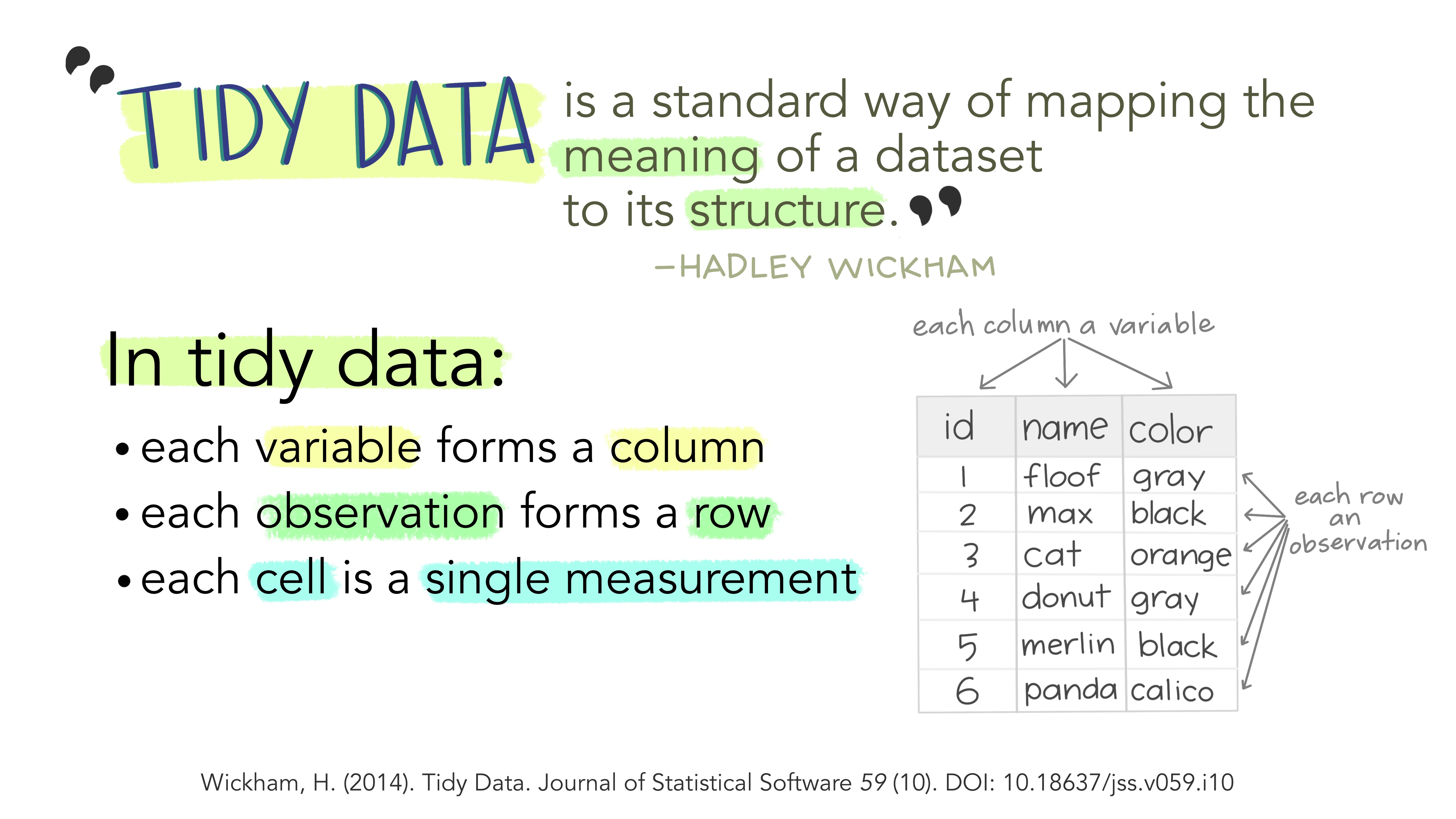
(2) Tidy Data (Wickham 2014).
(3) Ten Simple Rules for Reproducible Computational Research (Sandve 2013).
35.1 Protecting and nurturing your data
We care about the data, the data are our guide through this world. It is therefore very important to ensure the integrity of our data. Kate Laskowski learned this all too well, when her collaborator messed with her data set. In the required video below, she outlines the best practices to ensure the integrity of your data, both against unscrupulous collaborators, or, more likely, minor mistakes introduced in the process of data collection and analysis.
FIGURE 35.1: Kate Laskowski on data integrity (6 min and 06 seconds).
35.2 Data in spreadsheets
Data are most often stored in spreadsheets, or sometimes in databases. An important rule for reproducible data analysis is that data should be entered in a spreadsheet and then untouched. Instead of modifying data in a spreadsheet, we should develop scripts to process and filter the data. This ensures that we can honestly share exactly what we did and reproduce our analysis from raw data to final product.
35.2.1 Entering data into spreadsheets
A critical part of conducting a study is knowing what you are measuring, how you are measuring it, how you’re entering it and what else you might want to know.
If you are collecting your own data, or you are in on the ground floor of the initial data collection phase of a study, you should spend a few hours reflecting on what your spreadsheet should look like, and then take a handful of data and then revisit and restructure as necessary. In doing so, take the guidance in this section, largely lifted from (Broman and Woo 2018), into account. You’ll thank me later!!!
🧵10 fun facts about my paper with @kara_woo on Data Organization in Spreadsheets https://t.co/QFV0Dip1BJ
— Karl Broman (@kwbroman) November 12, 2020
35.2.1.1 Be consistent and deliberate
You should refer to a thing in the same thoughtful way throughout a column. Take, for example, gender as a nominal variable.
A bad organization would be: male, female, Male, M, Non-binary, Female.
A good organization would be: male, female, male, male, non-binary, female.
A just as good organization would be: Male, Female, Male, Male, Non-binary, Female.
🤔 Why? 🤔 Because if we are doing an analysis of say gender discrimination we don’t want males and Males to represent different groups.
The advice above also holds for dates and missing values.
The most common convention for dates is: YYYY-MM-DD.
The most common convention is to leave cells empty if you don’t have it yet, and fill them with
NAif you will never get that data point.
35.2.1.2 Use good names for things
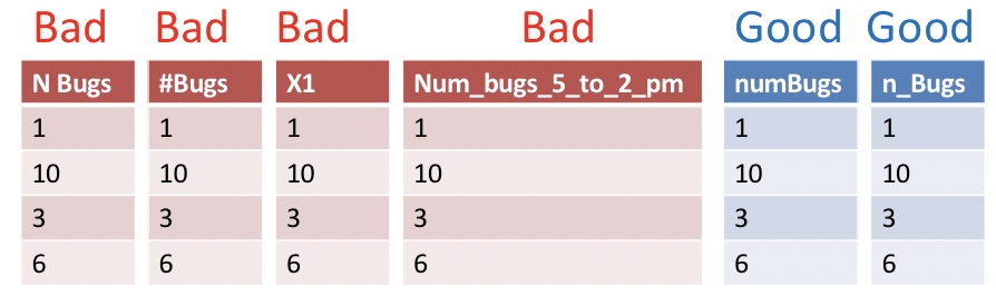
Names should be concise and descriptive. They need not tell the entire story. For example, units are better kept in a data dictionary than column name.
🤔 Why? 🤔 You don’t want to keep typing long awkward things in R but you do want variable names to convey meaning you can instantly recognize.
35.2.1.3 Make a data dictionary
What is a data dictionary, you ask? All the TMI that you would otherwise put in your overly complex column names. So, each row should correspond to a variable in the main data file, and each column should be additional info. For example, columns could be name, description, type, unit,range_or_values, etc…
🤔 Why? 🤔 You want to have this information easily accessible without gumming up your data sheet.
35.2.1.4 Do Not Use Font Color or Highlighting as Data
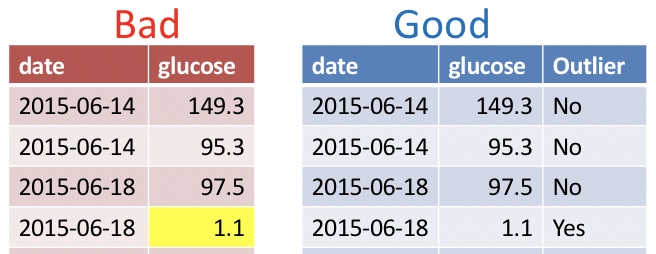
You may be tempted to encode information with bolded text, highlighting, or text color. Don’t do this! Be sure that all information is in a readable column.
🤔 Why? 🤔 These extra markings will either be lost or add an extra degree of difficulty to your analysis. Reserve such markings for the presentation of data.
35.2.1.5 No values should be implied.
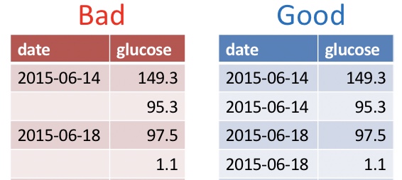
Never leave an entry blank as “shorthand for same as above”. Similarly, never denote the first replicate (or treatment, or whatever) by its order in a spreadsheet, but rather make this explicit with a value in a column.
🤔 Why? 🤔 Data order could get jumbled and besides it would take quite a bit of effort to go from implied order to a statistical analysis.
35.2.1.6 Backup your data, do not touch the original data file and do not perform calculations on it.
Save your data on both your computer and a locked, un-editable location on the cloud (e.g. google docs, dropbox, etc.)
🤔 Why? 🤔 Your data set is valuable. You don’t want anything to happen to it. It also could allow you to ensure that your collaborators (and/or former house-mates) did not manipulate the data.
35.2.2 Dealing with (other people’s) data in spreadsheets
We are often given data collected by someone else (collaborators, open data sets etc). If we’re lucky they did a great job and we’re ready to go. More often, they did ok and we have a painful hour to a painful week ahead of us as we clean up their data. Rarely, their data collection practices are so poor that their data are not useful.
In this course we will cover some basic data wrangling tools to deal with ugly datasets, but that is not a course focus or course goal. So, our attention to this issue will be minimal. If you want more help here, I suggest part II of R for Data Science (Grolemund and Wickham 2018).
35.2.3 Saving data
It’s best practice to save data as a lightweight, flat file like a .csv. Excel allows you to save datasets as a csv! But if you really want to use .xls or .xlsx format you can. Just be aware that some features, especially those I wanted you to avoid, above, may not work well once imported into R.
35.2.4 Organizing folders
Make life easy on yourself by giving each project its own folder, with sub-folders for data, figures, code, and writing. This makes analyses easy to share and reproduce.
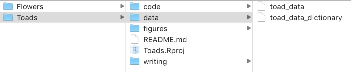
FIGURE 35.2: Example folder structure
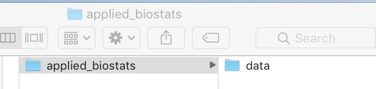
I highly recommend treating this course as a project, so make a folder on your computer called applied_biostats and a folder in there called data. If you do this, your life will be better. You might even want to do one better and tret each class session as a project.
35.3 Loading A Spreadsheet into R
Getting data into R is often the first challenge we run into in our first R analysis. The video (Fig: 35.3) and text below should help you get started.
FIGURE 35.3: Getting data into R (5 in and 10 seconds).
Ideally, your data are stored as a .csv, and if so you can read data in with the read_csv() function. R can deal with other formats as well. Notably, using the function readxl::read_excel() allows us to read data from Excel, and can take the Sheet of interest as an argument in this function.
Here’s an example of how to read data into R.
To start we open Toads.Rproj by either
- Opening RStudio by opening
Toads.Rprojor - Clicking
Fileand navigating toOpen projectonce RStudio is open.
library(tidyverse)
toad_data <- read_csv(file = "data/toad_data.csv")
Opening Toads.Rproj tells RStudio that this is our home base. The bit that says data/ points R to the correct folder in our base, while toad_data.csv refers to the file we’re reading into R. The assignment operator <- assignins this to toad_data. Using tab-completion in RStudio makes finding our way to the file less terrible. But you can also point and click your way to data (see below). If you do, be sure to copy and paste the code you see in the code preview into the script so you can recreate your analysis..
35.4 Tidying messy data
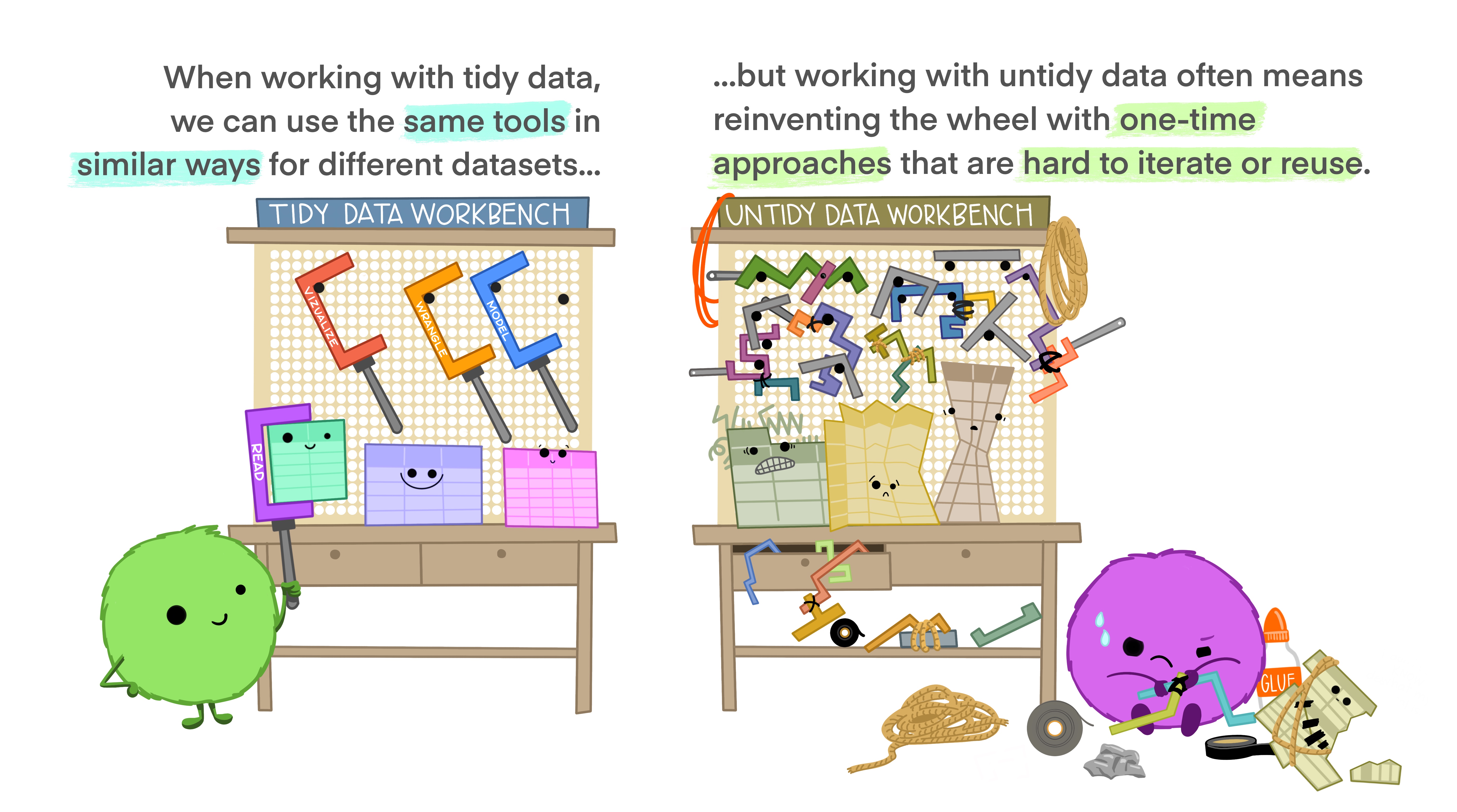
FIGURE 35.4: Tidy tools require tidy data
Above, we said it is best to keep data in a tidy format, and in Section 2.2.2 we noted that Tidyverse tools have a unified grammar and data structure. From the name, tidyverse, you could probably guess that tidyverse tools require tidy data – data in which every variable is a column and each observation is a row. What if the data you loaded are untidy? The pivot_longer function in the tidyr package (which loads automatically with tidyverse) can help! Take this example dataset, about grades in last year’s course.
## # A tibble: 2 × 4
##   last_name first_name exam_1 exam_2
##   <chr>     <chr>       <dbl>  <dbl>
## 1 Horseman  BoJack       35     36.5
## 2 Carolyn   Princess     48.5   47.5
This is not tidy. If it were tidy each observation would be a score on an exam. So we need to move exam to another column. We can do this!!!
tidy_grades <-pivot_longer(data = grades, # Our data set
             cols = c(exam_1, exam_2),    # The data we want to combine
             names_to = "exam",           # The name of the new column in which we put old names.
             values_to = "score"          # The name of the new column in which we put the values.
             )

tidy_grades
## # A tibble: 4 × 4
## last_name first_name exam score
## <chr> <chr> <chr> <dbl>
## 1 Horseman BoJack exam_1 35
## 2 Horseman BoJack exam_2 36.5
## 3 Carolyn Princess exam_1 48.5
## 4 Carolyn Princess exam_2 47.5This function name, pivot_longer, makes sense because another name for tidy data is long format. You can use the pivot_wider function to get data into a wide format.
Learn more about tidying messy data in Fig. 35.5:
FIGURE 35.5: Tidying data (first 5 min and 40 seconds are relevant).
Assignment
The assignment is to be turned in on canvas it has questions revolving around.
Identify a dataset for your project here. Explore the data… Does it follow best practices in spreadsheet setup? Explain why or why not.
Quiz questions that are the same as those below. If you try them first here, you’ll be sure to enter the right answers on canvas.
35.5 Functions covered in Handling data in R
All require the tidyverse package
read_csv(): Reads a dataset saved as a .csv into R.
readxl::read_excel(): Reads a dataset saved as a .xlsx into R. You can also specify the sheet with sheet =.
pivot_longer(): Allows use to tidy data.
pivot_wider(): Allows use to go from tidy to wide data.
35.5.1 tidyr cheat sheet
There is no need to memorize anything, check out this handy cheat sheet!
](https://raw.githubusercontent.com/rstudio/cheatsheets/main/pngs/tidyr.png)
FIGURE 35.6: download the tidyr cheat sheet
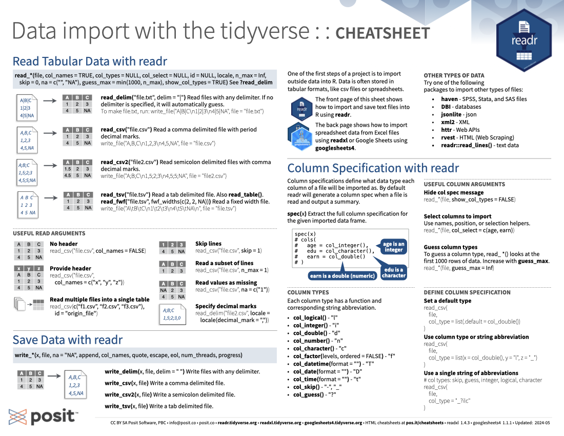
35.5.2 importing data cheat sheet
There is no need to memorize anything, check out this handy cheat sheet!
FIGURE 35.7: download the importing data cheat sheet